Probability Theory
中英双语随机使用,目的是为了让自己看懂,比较informal的lecture note,见谅。
4 Probability TOOLS
Distirbutive Law for Expectation
Tail Estimates
Monte Hall Problem
3 closed doors. Behind one door is a car, while the other 2 doors each has a donkey behind it.
First the guest pick a door, then Monte opens a different door which has a donkey. Monte ask the guest:"Would you like to change your choice?"
P=(U.p)
直观认为的\(\frac{1}{2}\)是先开门后选的结果,真实的概率应该是\(\frac{2}{3}\)
100doors, 只有一个有车,98 revealed, 胜率为99%
Birthday Paradox
n random people, how likely is it to have 2 people with the same birthday?
考虑没有两个人生日相同的情况
\(\frac{365\cdot 364 \cdot \cdot \cdot (365-n+1)}{365^n}\)
When we calculate, use the approximation \(1-x=e^{-x}\)
P=1-\((1-\frac{1}{365})\cdot\cdot \cdot (1-\frac{n-1}{365})\)
=1-\(e^{-\frac{n(n-1)}{2\cdot 365}}\)
Online Auction Problem
Sell a ticket to n=\(10^6\) interested buyers
A stream of distinct offers \(x_1,x_2,...,x_n\) you have to make the decision at real time. You want to maximize the probability pf accpeting the highest offer.
Strategy K 1)skip first k offers, the maxium in first k is MAX 2)Accept \(x_j\) if j is the first j satisfying \(x_j>MAX\)
U is the set of all permutations(排列)of {1,2,...,n} (n!)
T describe the case that one succeed
\(T_j=(n-1)!\frac{k}{j-1}\) (n-1)!考虑第n个最大,分数考虑条件(2)
\(P=\frac{\Sigma T_j}{n!}\)
\(H_n=1+\frac{1}{2}+...+\frac{1}{n}=lnn+C\)
\(P=\frac{k}{n}(lnn-lnk)\)
Basic Volcabulary for Graph
multiset is like a set except its members need not be distinct.
Def of multiset: a set together with a function that assigns to each member of the set a positive integer or \(\infin\)(called multiplicity)
图 graph 点 vertices 边 edge
A simple graph G is a pair of set (V,E). E is edege. Each element of E is a subset of size two of V.
Multigraph(graph with repeated edges)
|V|=number of vertices=the order of G
Ramsey numbers
The Union Bound
Among 6 people, there must exist either 3 mutual friends, or 3 nutual strangers
Proof:
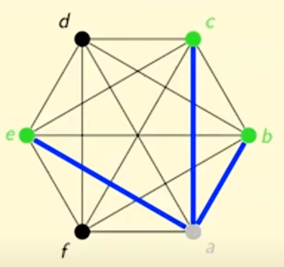
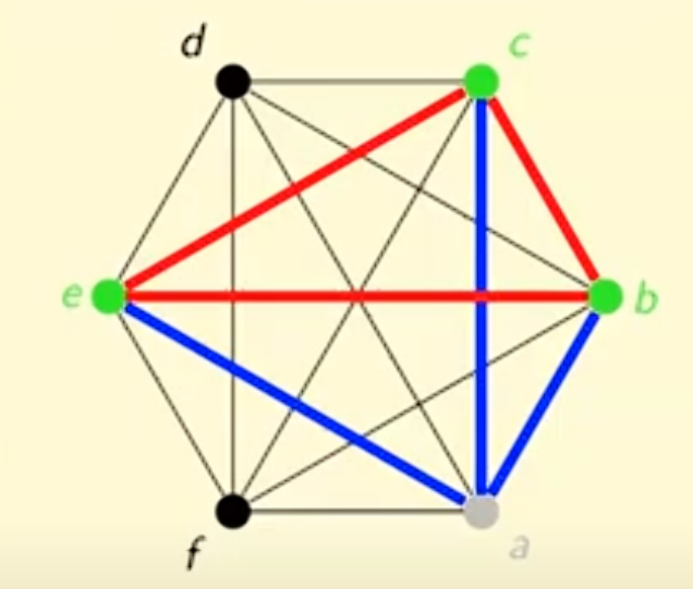
If you color the edges of K5 red and blue arbitraryly, then you are not guaranteed a red K3 or blue K3
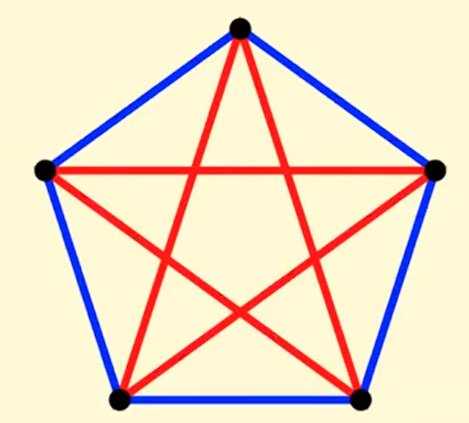
Define Ramsey Number:
Chain Rule
这个法则对于用条件概率计算总概率很有用
\(Pr(S_1\cap S_2\cdot\cdot\cdot\cap S_m)=Pr(S_1)Pr(S_2|S_1)Pr(S_3|S_2\cap S_1)\cdot \cdot Pr(S_m|S_1\cap \cdot \cdot S_{m-1})\)
特殊情形:\(S_k \subset S_{k-1} \cdot \cdot \cdot \subset S_{1}\)
此时\(Pr\{S_1\cap S_2\cdot \cdot \cdot \cap S_m\}=Pr\{S_1\}Pr\{S_2|S_1\}Pr\{S_3|S_2\}\cdot \cdot Pr\{S_m|S_{m-1}\}\)
Permutation
P=(U,p) where U is the set of all permutations, p(\(\sigma\))=1/|U| for all \(\sigma \in U\)
For each \(1\leq i \leq n\), let \(L_i(\theta)=\) length of cycle containing i.
Q:Probability
Q: What is the probability of 1 being in a cycle of length s?
Lemma:Pr(\(L_1=s\))=\(\frac{1}{n}\) for any s\(\in\){1,...,n}.
Proof:
Step1
Pr{\(L_1>s\)|\(L_1>s-1\)}=\(\frac{n-s}{n-s+1}\)
解析:
假设这个循环从1开始。为了得到这个概率表达式,我们可以考虑一个循环的前s位,由于\(L_1>s-1\),必有前s个点各不相同。\(L_1\)是否大于s取决于第s+1位是否又回到了1。如果在第s+1位回到了1,那么就有\(L_1=s\)。
下面我们考虑第s+1位的元素又多少种可能性。
第一种可能性又回到了1,这时\(L_1=s\)
第二种可能性不回到1,则这一位只能选择除了循环的前s位(包含1)的所有数,即有n-s种选择。
于是总共有n-s+1种选项,能选的是n-s(第二种情况)
Step2
Pr{\(L_1\)=s}=\(\frac{n-1}{n}\frac{n-2}{n-1}\cdot \cdot \cdot\frac{n-s+1}{n-s+2}\frac{1}{n-s+1}=\frac{1}{n}\)
解析:
我们可以使用Chain Rule来计算Pr{\(L_1>s-1\)}的大小。因为\(L_1>s \subset L_1>s-1\),我们可以使用特殊情形的。
回忆:P(AB)=P(A)P(B|A) 在这里我们令\(L_1>s-1\)作为事件A,因为它的概率很好求;令B为\(L_1=s\)
于是\(Pr(L_1>s-1)=\frac{n-1}{n}\frac{n-2}{n-1}\cdot \cdot \cdot\frac{n-s+1}{n-s+2}=\frac{n-s+1}{n}\)
\(Pr(L_1=1|L_1>s-1)=\frac{1}{n-s+1}\) 详见step1的“第一种可能性”
代入之后即可算出概率。
Q:Expectation
继承原始的题目条件,Let X be the random variable X(\(\sigma\))=# of cycles in \(\sigma\)'s cycle repesentation.
Q:What is E(X)?
\(\sigma=(3,5,1,4,2)\) contains cycle (2,5) and (3,4,1) \(L_1(\sigma)=3\) and \(L_5(\sigma )=2\)
Note that \(\Sigma_{i=1}^{n}\frac{1}{L_i(\sigma)}=\frac{1}{2}\cdot 2+\frac{1}{3}\cdot 3=2\)
From this we know that X=\(\Sigma_{i=1}^{n}\frac{1}{L_i(\sigma)}\) is the number of cycles.
注释:每一个长度为s的cycle在上面的算式中都可以得出一个\(s\cdot \frac{1}{s}=1\),因此我们可以这样断言。
E(X)=\(E(\Sigma_{i=1}^{n}\frac{1}{L_i(\sigma)})\)
因为在一个排列里n个元素地位是平等的,所以我们有\(E(L_1)=\cdot \cdot \cdot =E(L_i)\) 于是\(E(X)=nE(\frac{1}{L_1(\sigma)})\)
\(E(\frac{1}{L_1})=\Sigma_{s=1}^{n}P(L_1=s)\frac{1}{s}=\frac{1}{n}\Sigma_{s=1}^{n}\frac{1}{s}\)
Harmonic Number(调和级数):\(\Sigma_{s=1}^{n}\frac{1}{s}=H_n\)
E(X)=nE(\(\frac{1}{L_1}\))=\(H_n\)
(Q2配合下面一条食用)
Finding My Pet
这个问题也可以抽象成找permutation中的cycle
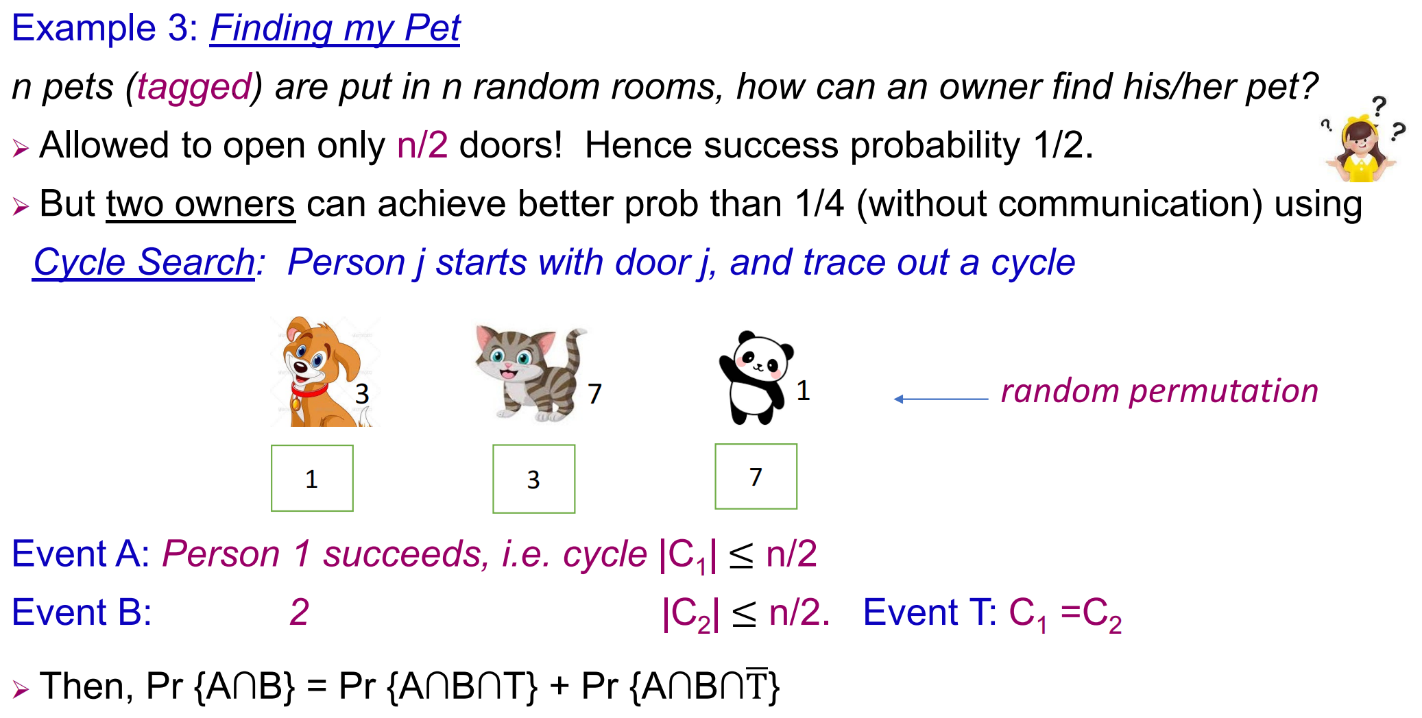
我们只需要关心这个cycle的大小和\(\frac{n}{2}\)的关系即可,如果\(\leq \frac{n}{2}\)的话,就成功了。

P(|\(C_i\)|=j)=\(\frac{1}{n}\)
\(B\cap T\)意味着两个cycle完全相同,所以2也在\(C_1\)中就等价于满足B。
\(C_1\)我们已经知道有j个不同的元素,而且有1。于是剩下的元素有j-1个坑位,
Random Variables
Random Variable Expectation的定义以及重要理论
Law of linear Expectation
$X=C_1X_1+C_2X_2+C_nX_n $
Then E(X)=\(\Sigma_i C_i E(X_i)\)
(新)Conditional Expectation
Random Variable X and Event T, u是各种可能的情况(事件)
E(X|T)=\(\frac{\Sigma_{u\in T}p(u)X(u)}{P(T)}\) if P(T)>0
当P(T)=0 E(X|T)=0
Distributive Law for 条件概率
X is random variable, U is the DISJOINT union of \(W_1,W_2,\cdot \cdot W_n\)
E(X)=\(\Sigma_i P(W_i)E(X|W_i)\)
Variance
Variance:Var(X)=\(E((X-E(X))^2)\)
Standard Deviation of X: \(\sigma(X)=\sqrt{Var(X)}\)
Fact:\(Var(X)=E(X^2)-(E(X))^2\)
独立随机变量
X.Y are independent if P(X=x,Y=y)=P(X=x)P(Y=y), in other words P(X=x|Y=y)=P(X=x)
If X,Y are independent
Thm1
E(XY)=E(X)E(Y)
Thm2
Var(X+Y)=Var(X)+Var(Y)
\(Var(X+Y)=E(X^2+2XY+Y^2)-(E(X+Y))^2\)
\(=E(X^2)+2E(X)E(Y)+E(Y^2)-E(X)^2-2E(X)E(Y)-E(Y)^2\)
对比?
Geometric Distribution
扔一枚硬币,正面朝上的概率为p,X是第一次扔出来正面的次数。
E(X)
E(X)=p\(\cdot 1+(1-p)E(X+1)\) 分类讨论第一次是否成功来计算期望。
由于E(X+1)=E(X)+1我们可以轻松算出E(X)=\(\frac{1}{p}\)
Var(X)
\(Var(X)=E(X^2)-(E(X))^2\)
\(E(X^2)=p\cdot 1+(1-p)\cdot E((X+1)^2)\)
\(E((X+1)^2)=E((X^2+2X+1))=E(X^2)+2E(X)+1\) then substitute it to the equation.
We have \(Var(X)=\frac{1-p}{p^2}\)
Tail Estimates
Markov's Inequality
X是一个非负的随机变量,then for any c>0, P(X>cE(X))<\(\frac{1}{c}\)
另一种形式:P(X>A)<\(\frac{E(X)}{A}\)
If E(X)=0, 那么所有X均为0,不等式显然成立
If E(X)>0, then E(X)=\(\Sigma p(u)X(u)>?\)
进行两步缩小:
第一步,只保留X>cE(X)
第二部,把这些留下来的X的期望全缩小到cE(X)
于是\(E(X)>P(X>cE(X))cE(X)\),两边约掉期望即可证毕。
Chebyshev's Inequality
For any c>0, \(P(|X-E(X)|>c \sigma(X))<\frac{1}{c^2}\)
另一种形式: \(P(|X-E(X)|>A)<\frac{Var(X)}{A^2}\)
\(|X-E(X)|>c \sigma(X)\) 等价于 \((X-E(X))^2>c^2 Var(X)\)
平方之后可以转换为Var(x),不然|X-E(X)|的期望无意义。
Use Markov's Inequality \(P((X-E(X))^2>c^2 Var(X))<\frac{E((X-E(X))^2)}{c^2 Var(X)}=\frac{1}{c^2}\)
Greedy Clique
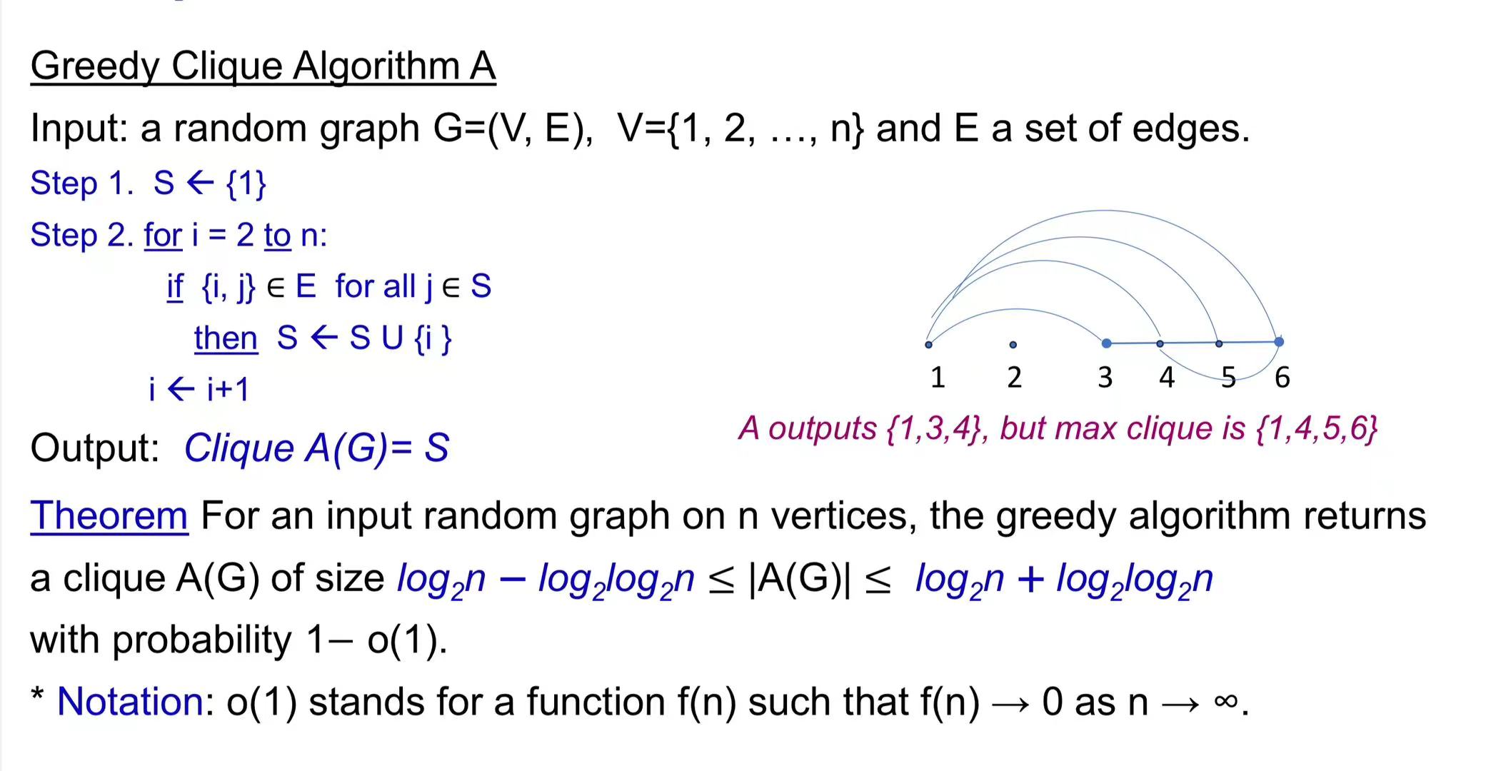
Upper Bound
p(\(|A(G)|>\log_2 n+\log_2\log_2n\))=o(1)
Let \(K=\log_2 n+\log_2\log_2n\) for \(2\leq i \leq n\).
\(T_i\) repesent the algorithm selects vertex i(初始给的图里的序号) as the K-th(选出的图里面的序号) vertex to join S.
Distributive Law: \(P(|S|>K)=\Sigma_{2\leq i \leq n}P(T_i)P(|S|>K|T_i)\)
至于为什么从2开始?因为1原先就在图里,无需算法选择。
\(P(|S|>K|T_i)\leq (n-i)\frac{1}{2^k}\leq\frac{n}{2^k}\)
解析:
如果S中已经有了k个点,那么下一个点想要加入必须和已经有的这k个都相连。这个概率就是\(\frac{1}{2^k}\)。
回忆Union Bound,一堆事件的“至少一个发生”的概率,不会超过它们各自发生的概率之和。
[ P(A_1 A_2 A_n) P(A_1) + P(A_2) + + P(A_n) ]
这个算法已经遍历了前i个点,因此我们能选的点就是剩下的n-i个。再用Union Bound,就得出了小于(n-i)乘以每一个点被加入的概率。
因此P(|S|>k)\(\leq \frac{n}{2^K}\Sigma_{2\leq i\leq n}P(T_i)\leq \frac{n}{2^K}\)
\(2^K=n\cdot \log_2 n\)
所以P(|S|>K)\(\leq \frac{1}{\log_2 n}=o(1)\)
Lower Bound
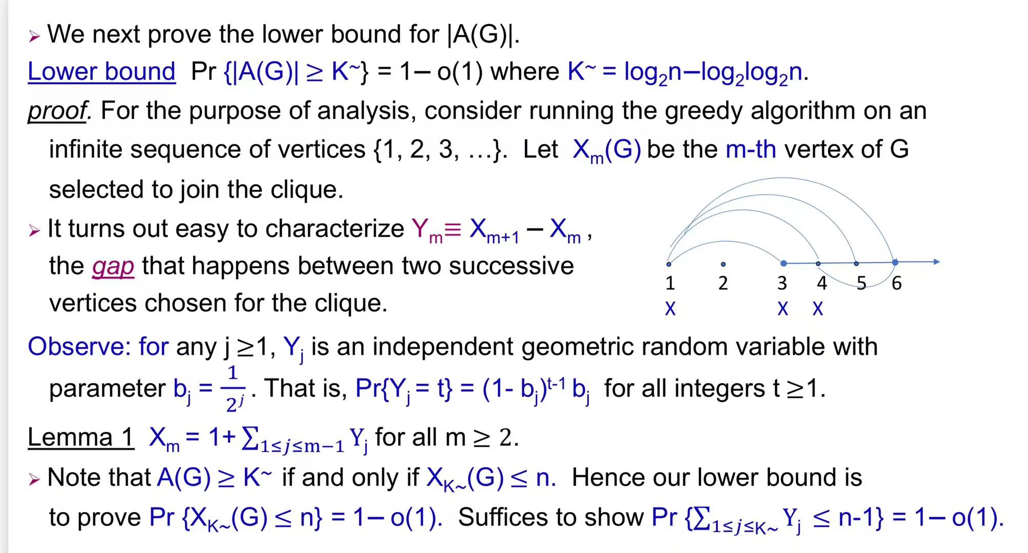
\(X_m(G)\)来表示G(算法生成的)第m个点。Y用来刻画前一个被选中的和后一个被选中的点之间的距离。
\(P(Y_j=t)=(1-b_j)^{t-1}b_j\) \(Y_j=t\)表示第j+1个加入的和第j个之间的间隔是t。\((1-b_j)^{t-1}\)刻画j之后的t-1个都不行,\(b_j\)刻画第j+1个加入的。
Lemma1:\(X_m\)就是初始值1加上所有的变化量Y
A(G)\(\geq K\):选出来的图至少有K个点。这个说法等价于,选到第K个点的时候,还可以继续选。也就是说第K个点的编号并没有超出n,即\(X_k(G)\leq n\)。
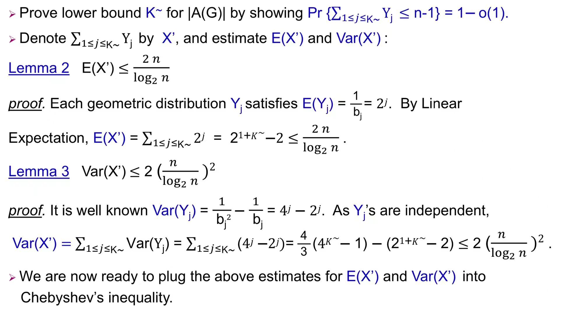
解析:记\(\Sigma_{1\leq j \leq K}Y_j=X'\)
Lemma2: \(Y_j\) 是现在有j个点,再添加一个点需要经过的间隔的期望。由于下一点就能加入图的概率是\(b_j=\frac{1}{2^j}\),所以我们可以把它看成一个几何分布。
E(X)=\(\frac{1}{p}\)(几何分布性质)于是\(E(Y_j)=\frac{1}{b_j}=2^j\)
直接根据期望能够线性相加,然后放大即可
Lemma3:\(Y_j\)相互独立,因为前一个点经过多少间隔走到下一个符合条件的点,不会互相影响
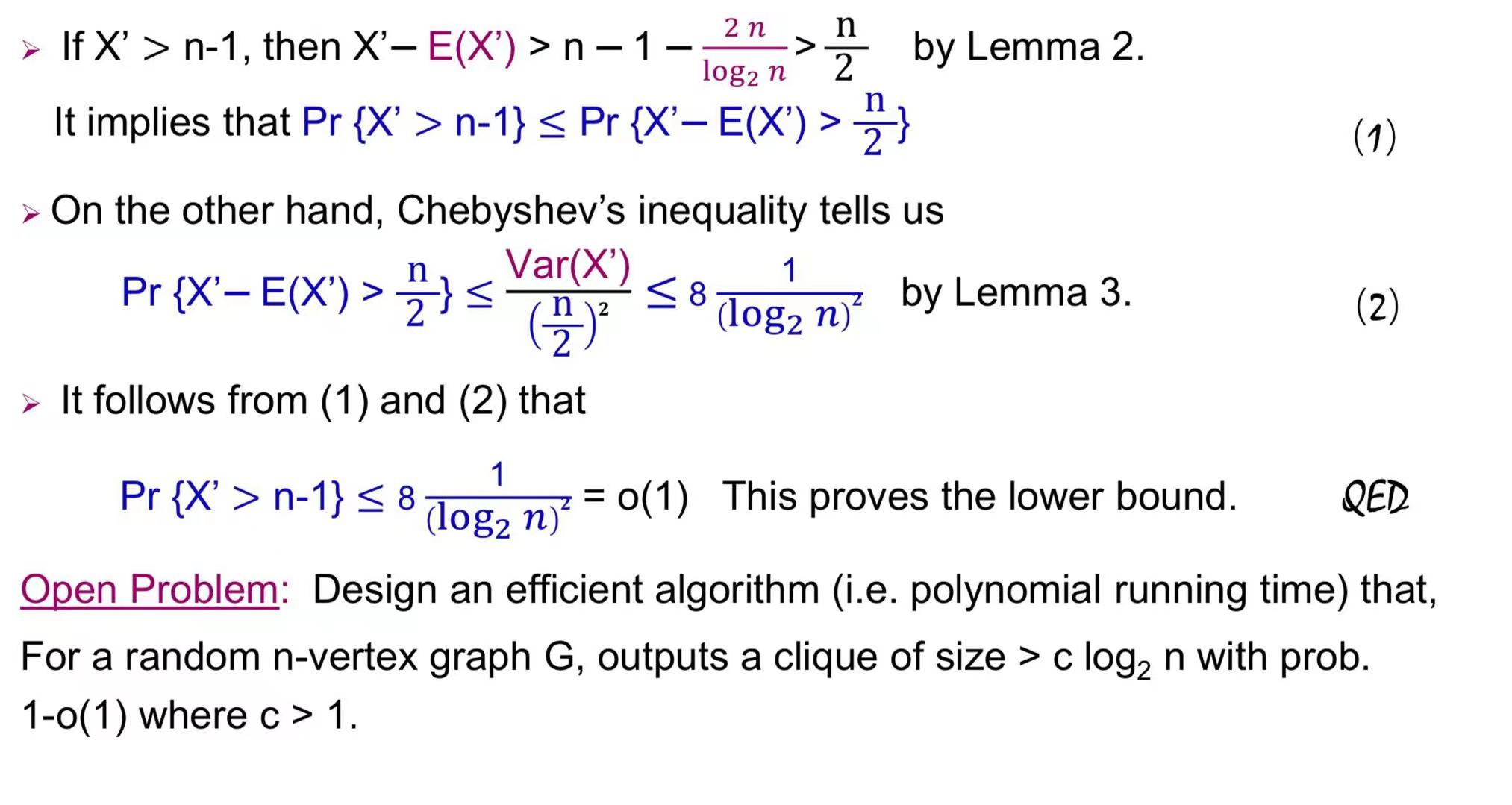
\(2(\frac{2}{3}(\frac{n^2}{(\log_2n)^2}-1)-\frac{n}{\log_2n}+1)\)
显然\(a=\frac{n}{\log_2 n}>1\)
如果我们要\(\frac{2}{3}a^2+\frac{1}{3}-a\leq a^2\) 只需要 \(-a^2-3a+1 \leq 0\),a满足这个要求
Monte Carlo
有一些函数我们并不能算出它们的积分,可以通过随机取样来估计积分值
Consider the integral: [ I={0}{1}e{-x^{3}}dx. ] - This integral has no closed - form solution. - Rewrite the integral as an expectation: [ I = [e{-U{3}}],U(0,1). ] - Generate (n) uniform random variables (U_1,,U_n) and compute: [ n={i = 1}{n}e{-U{i}^{3}}. ] - By Chebyshev’s inequality, (_n) converges to (I) quickly as (n).
A continuous random variable X is a random variable that can take on an uncountable number of values, typically over an interval of real numbers.
Definition: The probability density function (PDF) of a continuous random variable X is a function ( p(x) ) such that: [ P(a X b) = _{a}^{b} p(x) , dx ] for any interval ([a, b]). Properties of PDF: - ( p(x) ) for all ( x ). - The total area under the PDF curve is 1:
[ _{-}^{} p(x) , dx = 1 ]
Definition: The expectation (or expected value) of a continuous random variable ( X ) with PDF ( p(x) ) is: [ [X] = {-}^{} x p(x) , dx ] Definition: The variance of a continuous random variable ( X ) with PDF ( p(x) ) is: [ (X) = [(X - [X])^2] = {-}^{} (x - [X])^2 p(x) , dx ] Still holds: - Independence: ( p(x, y) = p(x) p(y) ). - Distributive law: ( (X) = (X^2) - ((X))^2 ). - Tail bounds: Markov’s inequality, Chebyshev’s inequality, Hoeffding’s inequality.
Sampling
问题:希望估计E[f(X)] with X~p
挑战:p可能过于复杂
关键:找到代理函数q(x)
Importance Sampling
关键:\(\int f(x)p(x)dx=\int f(x)\frac{p(x)}{q(x)}q(x)\) 我们可以选择已知的q(x),用q(x) 去生成 \(f(x)\frac{p(x)}{q(x)}\)
一次采样: [ N = {i=1}^{N} f(Y_i) , Y_i q. ] 这个公式表示通过重要性采样方法得到的估计值 (_N)。其中 (Y_i) 是从分布 (q) 中采样的随机变量,(f(Y_i)) 是某个函数,(p(Y_i)) 和 (q(Y_i)) 分别是目标分布和采样分布的概率密度函数。
unbiased 性质,一个估计量在多次重复抽样中的平均值接近于所要估计的参数的真实值: [ [_N] = = f(y)p(y) , dy = I. ]
方差:How many samples do we need to estimate ( [f(X)] ) within an accuracy ( ) with probability at least ( 1 - )?
Chebyshev's inequality: [ | ] , ]
The variance depends on the choice of ( q ): [ (_N) = ( , dy - I^2 ). ]
Reject Sampling
我们在一个给定区域内用已知函数进行采样,并判断采样点是否符合要求,不符合要求就丢弃。
对于已知采样函数,必须将所要求的PDF图像包含。
f(x)是想要估计的概率密度函数,g(x)是我们已知的,我们必须找到一个常数C使得\(Cg(x)\geq f(x)\)
Buffon's Neddle
平行线间距为d,针的长度l小于d。中点到最近的线的距离为x,针与直线的夹角为\(\theta\)。
\(0\leq x\leq \frac{d}{2}\), \(0 \leq \theta \leq \frac{pi}{2}\)
假设x,\(\theta\) 都是完全随机分布。下面是它们各自的概率密度函数。
\(x:f_x(x)=\frac{2}{d}\)
\(\theta:f_{\theta}(\theta)=\frac{2}{\pi}\)
Intersect if \(x \leq \frac{l}{2}sin\theta\)

\(f(x,\theta)=\frac{4}{\pi d}\)是概率密度函数。
P(\(x\leq \frac{l}{2}sin\theta\))=\(\int_{0}^{\frac{\pi}{2}}\int_{0}^{\frac{l}{2}sin\theta}\frac{4}{\pi d}dx d\theta=\int_{0}^{\frac{\pi}{2}}\frac{4}{\pi d}\frac{l}{2}sin\theta d\theta=\frac{2l}{\pi d}(-cos\theta)|_{0}^{\frac{\pi}{2}}=\frac{2l}{\pi d}\)
Shannon’s Theorem (Formal)
想要发送k个Bit,加密后为n位,解码为k位
Shannon’s theorem: The sender can reliably send messages of only about \(k = n(1 - H(p))\) bits within each block of \(n\) bits.
The term \(1 - H(p)\) is called the channel capacity: the maximum rate at which information can be transmitted reliably over the channel.
Theorem (Shannon’s Theorem)
For a binary symmetric channel with parameter \(p < 1/2\) and any constants \(\delta,\varepsilon > 0\), when \(n\) is sufficiently large: 1. For any \(k \leq n(1 - H(p)-\delta)\), there exist \((k, n)\) encoding and decoding functions such that the probability of decoding error is at most \(\varepsilon\) for every possible \(k\)-bit input message. 2. No \((k, n)\) encoding and decoding functions exist for \(k \geq n(1 - H(p)+\delta)\) such that the probability of decoding error is at most \(\varepsilon\) for a \(k\)-bit input message chosen at random.
名词定义
- Hamming distance dH(s,t):表示两个01字串有多少个不同的位数,eg \(d_H(1010, 0011)=2\).
- Let \(\mathcal{C}=\{c_1, c_2,\ldots, c_M\}\) be some arbitrary collection of distinct codewords with length \(n\) (we’ll call this a codebook). If we send \(c_i\) through the channel, the output is a random code \(\tilde{c}_i\).表示长度是n的所有加密后的n位字符串集合。
- By Chernoff’s bound, there is some \(\gamma\) so that with probability \(1 - \epsilon/2\), [(p - )nd_H(c_i, _i)(p + )n,] 为了表示:the distance between \(c_i\) and \(\tilde{c}_i\) is very likely to be close to \(np\).
- Choose \(\gamma>0\) as small as possible and define [(c_i)={c:|d_H(c_i, c)-np|n}.]
- So \(\tilde{c}_i \in \text{Ring}(c_i)\) with probability at least \(1 - \epsilon/2\).
- 成功的定义: \(\text{Success}_i(\mathcal{C})\) denote the event that \(\tilde{c}_i \in \text{Ring}(c_i)\), but \(\tilde{c}_i \notin \text{Ring}(c_j)\) for any \(j \neq i\). (In this case, upon receiving \(\tilde{c}_i\) we can be very confident about decoding it to \(c_i\).) ci只在Ring(ci)周围,不再任何其他的周围。
- So what we eventually want is a codebook where \(\mathbb{P}(\text{Success}_i(\mathcal{C}))\) is large for every \(i\).
lemma
The volume of a ring \(\text{Ring}(c_i)\) (the number of codewords with length \(n\)) is at most \(2^{(H(p) + \delta')n}\), where \(\delta' \to 0\) as \(n \to \infty\).
Based on the lemma, suppose we choose \(c_1,\ldots,c_M\) for \(M = 2^k\) uniformly at random. What is the probability that \(\text{Success}_i(\mathcal{C})\) holds for all \(i\)? (如果我们任意选M=\(2^k\)个c1,c2...cM(加密后字符串),k是初始的长度)
The proof will proceed in two main steps: 1. Step 1: Pick codewords uniformly at random, but twice as many as we will eventually need. We show such a random code is "good on average". 2. Step 2: After a derandomization step that picks the collection of codewords that is best on average, the "worst half" of the codewords are thrown away, yielding a collection of codewords where every code has a large probability of being correctly decoded.
第一步随机生成\(2*2^k\)个字串。我们要证明这些的平均值很好。第二步我们丢掉不行的,剩下的肯定必这个平均值更好。为什么要选\(2*2^k\)个,就是为了丢掉一半还剩下\(2^k\)个,剩下的那些就是我们最终想要的。
Proof of Shannon’s Theorem (Step 1)
- Now let’s choose \(\mathcal{C}\) randomly. Let \(M = 2\cdot2^k\) (this is twice as big as we want in the end), and let \(X_i\) be a uniformly chosen binary string in \(\{0, 1\}^n\). Let \(\mathcal{C}=\{X_1,\ldots,X_M\}\).
- Suppose now we pick a codeword \(i\) uniformly at random from \(\{1,2,\ldots,M\}\), and send it through the channel. What is the probability that we cannot decode it, i.e., that the event \(\text{Success}_i(\mathcal{C})\) does not occur?
注:这里的Successi(C)指的是第i个呗成功传输的概率。
Lemma (Step 1)
For \(\mathcal{C}\), \(i\) chosen randomly as described. Let \(\lambda_i(\mathcal{C}) = 1-\mathbb{P}(\text{Success}_i(\mathcal{C}))\).\(\lambda_i\)表示失败的概率。 [(_i()), n.] (Note: the expectation is taken over both the random choice of \(\mathcal{C}\) and the random choice of \(i\).)
Lemma (Step 1)
\(\mathbb{E}(\lambda_i(\mathcal{C}))\leq \epsilon\), \(\lambda_i(\mathcal{C}) = 1 - \mathbb{P}(\text{Success}_i(\mathcal{C}))\) and \(n\) is large enough. 失败的情况有两种,第一种是\(\tilde{c}_i \not\in \text{Ring}(c_i)\),第二种是\(\tilde{c}_i \in \text{Ring}(c_j)\) for some \(j \neq i\) - With probability at least \(1 - \epsilon/2\), \(\tilde{c}_i \in \text{Ring}(c_i)\). The main work is to show that the probability that \(\tilde{c}_i \in \text{Ring}(c_j)\) for some \(j \neq i\) is small.想要证明这两种失败概率很小。 - First, fix some arbitrary \(j \neq i\) and fix some arbitrary \(\tilde{c} \in \text{Ring}(c_i)\). - The probability that \(\tilde{c} \in \text{Ring}(c_j)\) is the same as the probability that \(c_j \in \text{Ring}(\tilde{c})\), which is just the "volume" of \(\text{Ring}(\tilde{c})\) divided by the volume of \(\{0, 1\}^n\). - The volume of a ring is at most \(2^{(H(p)+\delta')n}\). Thus [( (c_j))=(c_j ())^{(H(p)+'-1)n}(两volume相除).] - This is true for any \(\tilde{c}\) in \(\text{Ring}(c_i)\), and so we can deduce that [(_i (c_j)|_i (c_i))^{(H(p)+'-1)n}.]能写出条件概率是因为这个对any \(\tilde{c}\) in \(\text{Ring}(c_i)\)成立 - Now take a union bound, [ \[\begin{align*} \mathbb{P}(\text{Success}_i(\mathcal{C})\text{ does not occur})&\leq M2^{(H(p)+\delta'-1)n}+\epsilon/2\\ &=2^{1+(k/n + H(p)+\delta'-1)n}+\epsilon/2. \end{align*}\] ] ????为什么是M????? - Now take a union bound, [ \[\begin{align*} \mathbb{P}(\text{Success}_i(\mathcal{C})\text{ does not occur})&\leq M2^{(H(p)+\delta'-1)n}+\epsilon/2\\ &=2^{1+(k/n + H(p)-1+\delta')n}+\epsilon/2. \end{align*}\] ] - \(\delta' \to 0\) as \(n \to \infty\); - Since \(k/n < 1 - H(p)\)(这个是根据证明条件里面k的范围得出), it follows that \(k/n - H(p) + 1 + \delta' < 0\) for \(n\) large enough. The first term then goes to zero with \(n\), and so for \(n\) large enough, [ (_i())<.(第一类失败+第二类失败) ] - QED.
step 2
- Choose (n) large enough so that Lemma (Step 1) holds.
- Have ((i())) written out explicitly as an average:注意\(\lambda_i\)表示的是失败的概率。 [{}_{i = 1}^{M}_i().]
- There must be some choice of codebook (^*) which does better than average, i.e., for which (_{i = 1}^{M}_i(^*)). So we have found a codebook that is "good on average".
- So let (') be the codebook consisting of just the best half of the codewords in (^*): those with the smallest values of (_i(^*)). Then (_i(^*)) for all (c_i').????为什么是2\(\epsilon?\),不应该是\(\epsilon\)吗???丢掉容易失败的那一半,剩下的失败概率小于\(\epsilon\)
- So (') provides a good code with (2^k) codewords, and so it can be used as an ((k, n)) - encoding scheme.