老派自然语言处理之必要

Context-free Grammar

Basic Concepts

S: start symbol

T: non-terminals

x,y,1,2,3….: terminals

$\epsilon$ empty string

Derivations: A sequence of
steps where non-terminals are
replaced by the right-hand side
of a production rule in the CFG.

CFL L(G)

Every regular language is context-free.

Regex Examples:

b* : X-> $\epsilon$ | Xb

[cde] : Y-> c | d | e

S -> aSb | $\epsilon$ cannot be expressed by regex, because regex cannot express a string with a string with same amount of a and b.

L0

CFG covers more than we really want, but it is already useful for parsing.

eg. VP -> Verb NP “write a flight” do not make sense.

Non-CFL Example

$L={a^nb^nc^n|n>0}$

CNF (Chomsky normal form)

Definition: A CFG is CNF if it is $\epsilon$-free.

Explanation: Either A -> BC or A->a

Theorem: Any CFG can be converted into CNF. (eg.b*)

$$\begin{array}{l} S \to X \mid \epsilon \\ X \to XB \mid b\\ B \to b \end{array}$$

Parsing

Definition: syntatic parsing means mapping from a scentence to its parse tree.

CKY Parsing

First, convert grammar to CNF.

Then, dynamic programming.

function CKY-PARSE(words, grammar) returns table
  for j ← from 1 to LENGTH(words) do
    // 阶段 1: 处理长度 L=1 的子串
    for all {A | A → words[j] ∈ grammar}
      table[j-1, j] ← table[j-1, j] ∪ A
    
    // 阶段 2: 处理长度 L >= 2 的子串
    for i ← from j-2 down to 0 do
      for k ← i+1 to j-1 do
        for all {A | A → BC ∈ grammar and B ∈ table[i, k] and C ∈ table[k, j]}
          table[i, j] ← table[i, j] ∪ A

Non-terminal	Production Rules
S	$\to$ NP VP
NP	$\to$ Det Nom \	PropN
Nom	$\to$ Noun \	Noun Nom
VP	$\to$ Verb NP \	Verb
Det	$\to$ ‘the’ \	‘a’
Noun	$\to$ ‘book’ \	‘flight’
PropN	$\to$ ‘Houston’
Verb	$\to$ ‘booked’

Convert to CNF:

Non-terminal	Production Rules
S	$\to$ NP VP
NP	$\to$ Det Nom \	‘Houston’
Nom	$\to$ ‘book’ \	‘flight’ \	Noun Nom
VP	$\to$ Verb NP \	‘booked’
Det	$\to$ ‘the’ \	‘a’
Noun	$\to$ ‘book’ \	‘flight’
PropN	$\to$ ‘Houston’
Verb	$\to$ ‘booked’

the book booked

Apply CKY:

(0,1): Det

(1,2): Nom/Noun

(0,2): (0,1)+(1,2) NP -> Det Nom

(2,3): VP/Verb

(1,3): (1,2)+(2,3) 空

(0,3): (0,2)+(2，3) S -> NP VP

Latent Semantic Analysis

TD Matrix

document number |D|

vocab number |V|

|V|$\times$ |D|

每一个entry代表这个词在文件里出现的次数

$$\mathbf{W}_{td} = \begin{array}{c} \text{cat} \\ \text{dog} \\ \text{the} \end{array} \left[ \begin{array}{ccccccc} d_1 & d_2 & d_3 & d_4 & d_5 & d_6 & d_7 \\ 1 & 1 & 0 & 1 & 0 & 1 & 0 \\ 0 & 2 & 0 & 1 & 1 & 1 & 0 \\ 20 & 13 & 18 & 22 & 15 & 4 & 20 \end{array} \right]$$

Good: related words do appear together!

Bad: Related words “sometimes” appear together， the co-occurrence statistics might be sparse（矩阵中0很多）

SVD

• 目标： 不直接使用高维、稀疏的词-文档矩阵 ($W_{td}$)，而是为每个词汇 ($w$) 和文档 ($d$) 推断出一个低维的潜在向量 (Latent Vector, lv) 表示。
• 数学近似： 词 $i$ 与文档 $j$ 的关系 $W_{td}(i, j)$ 被近似为它们潜在向量的点积（并确保非负）： $$W_{td}(i, j) \approx \max(lv(w_i)^T lv(d_j), 0)$$
• $W_{td}$ 矩阵： 行是词汇，列是文档，单元格是词频或TF-IDF值。

$$W_{td} = U \Sigma V^T$$

矩阵	作用	描述
$U$	词表示矩阵	包含词汇的潜在向量表示（行）。
$\Sigma$	奇异值矩阵	对角矩阵，包含奇异值，用于确定降维时保留多少维度（即潜在语义的数量）。
$V^T$	文档表示矩阵	包含文档的潜在向量表示（列）。

保留最重要的k个奇异值——保留U的前K列，V的前K行

• 问题： SVD 产生的 $U$ 和 $V$ 矩阵是正交的，并且其元素可以包含负值。这与原始的 $W_{td}$ 矩阵是非负的特性不符，有时会降低模型结果的可解释性。SVD would pay too much attention to the high-freq words!

TF-IDF normalization

$$count'(i, j) = \text{tf}(i, j) \cdot \text{idf}(i)$$ $$\text{tf}(i, j) = \frac{\text{词 } i \text{ 在文档 } j \text{ 中出现的次数}}{\text{文档 } j \text{ 中的词总数}}$$

Smoothed版本，用于避免除以零和给予常见词语非零的得分：

$$\text{idf}(i) = \log\left(\frac{\text{文档总数} + 1}{\text{包含词 } i \text{ 的文档数} + 1}\right) + 1$$

逆文档频率 $\text{idf}(i)$ 衡量一个词 $i$ 在整个语料库中的普遍性或稀有性。它的核心思想是：一个词在越少的文档中出现，它就越具有区分度，其权重就应该越高。

EM Algorithm

GMM

mixture of gaussian distributions

隐变量 $z$（Latent Assignment）

• 定义： $z$ 是一个离散的隐变量，代表观测到的数据点 $x$ 是由哪个高斯分量 $c$ 生成的。
• 特点： 我们观察到数据 $x$，但不知道 $x$ 属于哪一个分量（即 $z$ 是隐藏的）。

生成一个数据点 $x$

1. 选择混合分量：

   $$p(z=c) = \pi_c$$
   • 首先，以概率 $\pi_c$ 选择一个高斯分量 $c$。$\pi_c$ 就是该分量的混合系数。

2. 从分量中采样：

   $$p(x|z=c) = \mathcal{N}(x; \mu_c, \sigma_c)$$
   • 一旦选择了分量 $c$，就从这个分量对应的高斯分布 $\mathcal{N}$ 中采样生成数据点 $x$。

求和

由于隐变量 $z$ 是我们不知道的，为了得到观测数据 $x$ 的总概率 $p(x)$，我们需要对 $z$ 的所有可能取值（即所有的分量 $c$）进行求和（边缘化）：

$$\begin{aligned} p(x) &= \sum_c p(x, z=c) \\ &= \sum_c p(x|z=c) p(z=c) \\ &= \sum_c \mathcal{N}(x; \mu_c, \sigma_c) \cdot \pi_c \end{aligned}$$

EM algo

GOAL: find $\theta$ to maximize log likehood of observed data.

$$\log p(X|\theta) = \log \sum_Z p(X, Z|\theta)$$

1. 随机初始化 (Random Initialization)

随机设定模型的初始参数 $\theta_0$。例如，在 GMM 中，就是随机设置每个高斯分量的初始 $(\pi_c, \mu_c, \sigma_c)$。

• 注意： E-M 算法保证收敛到局部最优解，因此初始化的选择会影响最终的结果。

2. 迭代直到收敛 (Iterate until convergence)

不断重复 E 步和 M 步

E 步 (Expectation Step): 猜测隐变量（$Z$）的隶属关系

• 公式： 计算 $q(Z) := p(Z|X, \theta_k)$。

$X$ 是观测数据，假设 $\theta_k$是对的，得到关于$Z$ 的最佳猜测分布 $q(Z)$
具体表现为每个数据点 $x_i$ 来自每个分量 $c$ 的概率：

$$\gamma_{ic} = p(z_i = c | x_i, \theta_k)$$
 $\gamma_{ic}$（Responsibility）

M 步 (Maximization Step): 精修模型参数（$\theta$）

假设现在$q(Z)$是真实的, 更新 $\theta$ 以最大化 $\sum_Z q(Z) \log p(X, Z|\theta)=\mathbb{E}_q[\log p(X, Z|\theta)]$
关键： 经过 E 步的转换，这个期望函数的形式通常简化为具有解析解（Closed-Form Solution），允许我们直接计算出最优的 $\theta$。

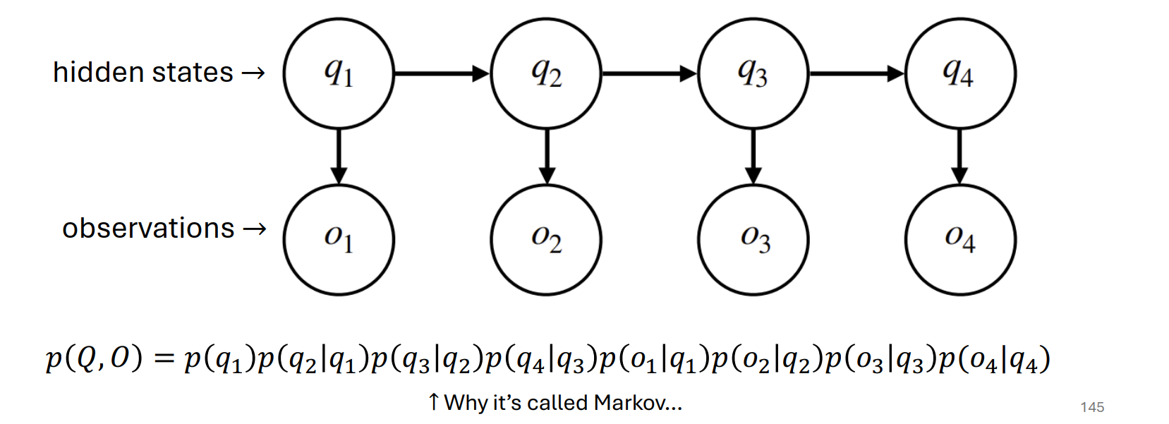
Hidden Markov Model (HMM)

Motivation task: position tagging, named entinity recognition.

inital probability: $\pi$

hidden states transfer:
$p(q2 \mid q_1) = a{q_1, q_2}$

emission probability: $b_i(o_k)$

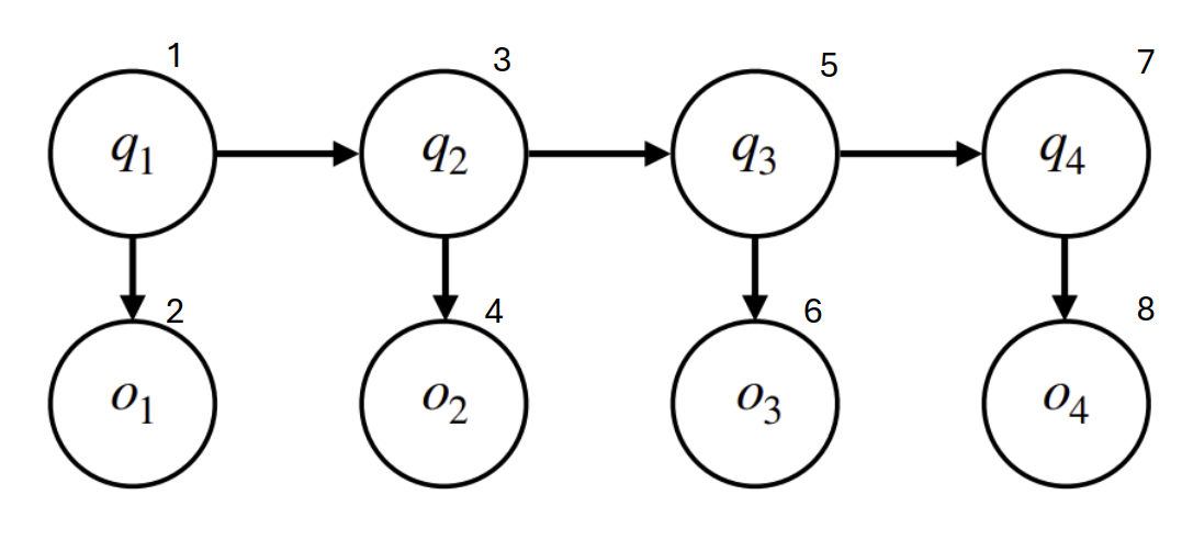
topology order: 先生成o在生成下一个q

marginal probability of an observation: $p(\mathbf{O})=\sum_{\mathbf{Q}} p(\mathbf{O}, \mathbf{Q})$.

N: number of hidden state Q

T：sequence length

路径总数 $(num tags)^{seqlen}=N^T$

每条路径计算成本 $O(T)$

总成本$O(TN^T)$

forward algorithm

$$p(o_{1:t}, q_t = j)\equiv\alpha(t, j) = b_j(o_t) \sum_{i} \alpha(t-1, i) a_{ij}\quad O(N)$$ $$\alpha(1, j) = \pi_j b_j(o_1)$$ $$p(\mathbf{O}) = \sum_{j} \alpha(T, j)$$

j一共有N个，算到T步需要算T次，一次N复杂度，所以是$O(N^2T)$

backward algorithm

$$p(O_{t+1:T} \mid q_t = i) = \sum_{j} [p(O_{t+2:T} \mid q_{t+1} = j) \underbrace{p(q_{t+1} = j \mid q_t = i)}_{A} \underbrace{p(o_{t+1} \mid q_{t+1} = j)}_{B}]$$ $$\beta(t, i) = \sum_{j} a_{ij} b_j(o_{t+1}) \beta(t + 1, j)$$ $$\alpha(t, i) \beta(t, i) = p(\mathbf{O}, q_t = i)$$

Vertibi——find the most probable q

$$\mathbf{Q}^* = \underset{\mathbf{Q}}{\operatorname{argmax}} \, P(\mathbf{Q} \mid \mathbf{O})$$ $$\underset{\mathbf{Q}}{\operatorname{argmax}} \, P(\mathbf{Q} \mid \mathbf{O}) = \underset{\mathbf{Q}}{\operatorname{argmax}} \, \frac{P(\mathbf{Q}, \mathbf{O})}{P(\mathbf{O})}$$

因为P(O)是观测到的常数

$$\underset{\mathbf{Q}}{\operatorname{argmax}} \, P(\mathbf{Q} \mid \mathbf{O}) = \underset{\mathbf{Q}}{\operatorname{argmax}} \, P(\mathbf{Q}, \mathbf{O})$$

表示在观测到序列的前 $t$ 个元素 $(\mathbf{O}_{1:t})$ 的条件下，所有以隐藏状态 $q_t = j$ 结尾的路径中，最大概率的那条路径的概率值：

$$\delta(t, j)=\max_{Q_{1:t-1}} p(\mathbf{O}_{1:t}, \mathbf{Q}_{1:t-1}, q_t = j)$$ $$\delta(t, j) = b_j(o_t) \max_{i} \delta(t - 1, i) a_{ij}$$ $$\delta(1, j) = \pi_j b_j(o_1)$$

Where do $\pi$ A ,B come from

Supervised learning: labeled data.

Unsupervised learning:

$$\log p(O|\theta) = \log \sum_Q p(O, Q|\theta)$$

DGM(Direct Graphical Model)

normalized property

For DAG, as long as each of the (separate) conditional distribution is a valid (normalized), then the joint distribution is normalized.

$$P(O, S, H, C) = P(O) \cdot P(S) \cdot P(H \mid O, S) \cdot P(C \mid S)$$

（这里 $O$=overweight, $S$=smoking, $H$=heart disease, $C$=cough）

我们对所有变量求和：

$$\sum_{O, S, H, C} P(O, S, H, C) = \sum_{O, S, H} \left[ P(O) P(S) P(H \mid O, S) \cdot \sum_{C} P(C \mid S) \right]$$

1. 对 $C$ 求和： 因为 $P(C \mid S)$ 是归一化的，所以 $\sum_{C} P(C \mid S) = 1$。

   $$\sum_{O, S, H} P(O) P(S) P(H \mid O, S) \times 1 = \sum_{O, S, H} P(O) P(S) P(H \mid O, S)$$

2. 对 $H$ 求和： 因为 $P(H \mid O, S)$ 是归一化的，所以 $\sum_{H} P(H \mid O, S) = 1$。

   $$\sum_{O, S} P(O) P(S) \times 1 = \sum_{O, S} P(O) P(S)$$

3. 对 $O$ 和 $S$ 求和： 因为 $P(O)$ 和 $P(S)$ 是独立的边缘分布，我们可以分别求和：

   $$\sum_{O} P(O) \cdot \sum_{S} P(S)$$

   由于边缘分布本身是归一化的：$\sum{O} P(O) = 1$ 且 $\sum{S} P(S) = 1$。

   $$1 \times 1 = 1$$

acyclic

A<->B

If I “set” P(A=0|B=0)=1, P(A=1|B=1)=1, P(B=1|A=0)=1, P(B=0|A=1)=1…

Basically B is 100% sure that A=B, while A is 100% sure that A!=B…

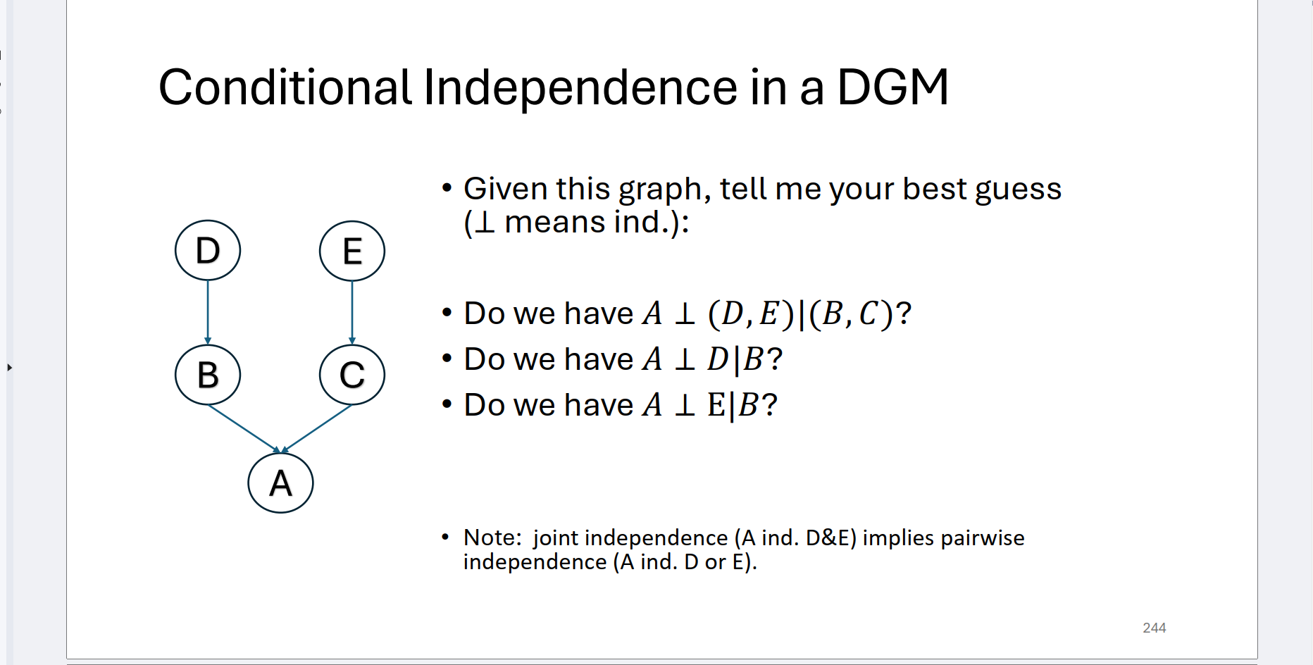
第一个的意思是：在已知 $B$ 和 $C$ 的条件下，$A$ 是否独立于 $D$ 和 $E$ 的联合集合？

答案：是是否

汇聚节点

A->B<-C 观测到B,AC不独立

D-连接 (d-connected) 的定义

(1) 汇聚节点条件 (Collider Rule): 路径 $U$ 上的每一个汇聚节点（Collider，即 $\rightarrow Z \leftarrow$ 结构中的 $Z$）都有后代位于观测集 $W$ 中**（包括 $Z$ 本身位于 $W$ 中）。

* **含义：** 汇聚节点上的信息流必须被观测到（或者其结果被观测到）才能被**打开**。

(2) 非汇聚节点条件 (Non-Collider Rule): 路径 $U$ 上的其他任何节点（非汇聚节点，即串联 $\rightarrow Z \rightarrow$ 或发散 $\leftarrow Z \rightarrow$ 结构中的 $Z$）都不在观测集 $W$ 中。

N-gram LM

Various applications of LM

Generation

• Auto-complete

• Speech-to-text

• Question-answering / chatbots

• Machine translation

• Summarization

Classification

• Authorship attribution

• Detecting spam vs not spam

• Grammar Correction

N-gram

Unigram LM

认为每一个词都是独立的，容易导致错误的句子和正确的句子概率一样$P_{unigram}(w_1 ... w_T) = P(w_1)P(w_2) ... P(w_T)$

Bigram LM 每两个词来考虑

Ngram LM

真实的概率 $P(w_{1:T}) = \prod_{t=1}^{T} P(w_t | w_{1:t-1})$

N-gram 模型假设一个词 $wt$ 的出现只依赖于它前面紧邻的 $N-1$ 个词，而不是全部的历史 $w{1:t-1}$。

$$P(w_t | w_{1:t-1}) \approx P_{ngram}(w_t | w_{t-N+1:t-1})$$

special tokens

\ end of scentence

\ out-of-vocabulary token

set word appear at least twice as vocabulary and others as \

How to get P？

MLE:

$$P_{tri}(\text{NLP} | \text{we study}) = \frac{count(\text{we study NLP})}{count(\text{we study } *)}$$

Problem: Sparsity, if we study NLP does not apper in the training corpus, then the probability will be 0.

add-k smoothing

$$P_{tri}(w_t | w_{t-2}w_{t-1}) = \frac{count(w_{t-2}w_{t-1}w_t) + k}{count(w_{t-2}w_{t-1}) + k|V|}$$

因为 Add-k 对所有 N-gram 都一视同仁地增加了 $k$，这可能会对高频 N-gram 的概率造成不必要的扭曲

Interpolation or backoff

线性插值公式： 将不同阶的 N-gram 模型的概率进行加权平均：

$$P_{tri}(w_t | w_{t-2}w_{t-1}) = \lambda_1 P_{tri}(w_t | w_{t-2}w_{t-1}) + \lambda_2 P_{bi}(w_t | w_{t-1}) + \lambda_3 P_{uni}(w_t)$$

回退： 如果 Trigram 计数为 0，则回退到 Bigram 模型 $P_{bi}$。

$$P_{tri-BO}(w_t | w_{t-2}w_{t-1}) = \begin{cases} P^*_{tri}(w_t | w_{t-2}w_{t-1}) & \text{if } count(w_{t-2}w_{t-1}w_t) > 0 \\ \alpha(w_{t-2}w_{t-1})P_{bi}(w_t | w_{t-1}) & \text{otherwise} \end{cases}$$

LM evaluation

PPL(Perplexity) 越低越好

$$PPL(W) = 2^{-l}, \quad \text{where } l = \frac{\log_2(P(W))}{token\_len(W)}$$

• $P(W)$ 是模型计算出的整个测试集句子的概率。
• $token_len(W)$ 是测试集中的词/token总数。

PPL does not involve actual generation. (衡量模型分配给已知测试数据的概率高低)

PPL cares more diversity than quality.

Example: If LM’s probability concentrate on a small set of very good
sentences, then the model’s PPL on a held-out set will be very bad.

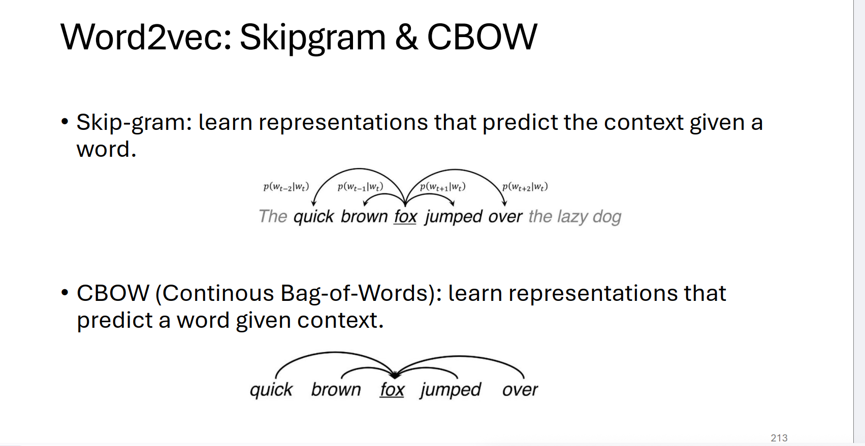
Word2Vec

parameters: input embedding W for context, output embedding U for prediction.

every row is a vector for a word.

Skipgram

objective:

$$p_{\theta}(\text{out} | \text{input}) = \frac{\exp(u_{\text{out}} \cdot w_{\text{input}})}{\sum_{v \in V} \exp(u_v \cdot w_{\text{input}})}$$

computation bottleneck: 分母takes $O(V)$ to compute.

solution：negative sampling

• 对于一个给定的中心词 $x$ 和一个上下文词 $y$（这是一个正例），我们希望模型预测它们是一对的概率高。
  • 我们随机抽取 $k$ 个负例 $y’$（非上下文词），希望模型预测 $x$ 和这些 $y’$ 不是一对的概率高。

$$\log \sigma(\mathbf{u}_y \cdot \mathbf{w}_x) + \sum_{i} \mathbb{E}_{y' \sim P_n} [\log \sigma(-\mathbf{u}_{y'} \cdot \mathbf{w}_x)]$$

符号	含义	解释
$\log \sigma(\mathbf{u}_y \cdot \mathbf{w}_x)$	正例项	希望最大化 $x$ 和真实上下文 $y$ 是一对的概率（点积越大，$\sigma$ 越大，$\log \sigma$ 越接近 0）。
$\log \sigma(-\mathbf{u}_{y’} \cdot \mathbf{w}_x)$	负例项	引入负号 $(-\dots)$，目的是希望最大化 $\sigma(-\mathbf{u}{y’} \cdot \mathbf{w}_x)$，这等价于最小化 $\sigma(\mathbf{u}{y’} \cdot \mathbf{w}_x)$。这迫使模型预测 $x$ 和非上下文 $y’$ 不是一对的概率高。
$P_n$	负采样分布	“$\mathbf{P}_n$ can be a unigram model.” 通常使用词汇的一元模型（Unigram Model）作为采样分布，即词 $v$ 被采样的概率与其在语料库中的频率相关。

Q1: 在 SGD 训练过程中，所有向量都会收敛到同一个值吗？为什么？

不会收敛到同一个值。

1. 目标函数的分母 (Softmax)： 分母 $\sum{v \in V} \exp(u_v \cdot w{\text{input}})$ 会计算输入词向量 $w_{\text{input}}$ 与词汇表中所有词的输出向量 $u_v$ 的相似度。这意味着，为了最大化上下文词的概率，模型必须学会在高维空间中将词语区分开来。
2. 上下文关系： 不同的词有不同的上下文。例如，“猫”的上下文通常是“抓”、“毛茸茸”，而“车”的上下文通常是“驾驶”、“轮胎”。模型会根据这些不同的统计关系，将具有相似上下文的词汇拉近，将不相似的词汇推远。

Q2: 拥有一个不同的输出嵌入矩阵 $U$ (Output Embedding) 是否有用？

角色分离 (Separation of Roles):

• $W$ (输入嵌入/中心词): 学习如何表示一个词，以便它能被用于预测其上下文。
• $U$ (输出嵌入/上下文词): 学习如何作为一个分类器或预测层的权重，来识别哪些词是中心词的上下文。

CBOW

$$p_{cbow}(x_t | x_{t-s} \dots x_{t+s}) = \frac{\exp(\mathbf{u}_{x_t} \cdot \frac{1}{2S}\sum_j \mathbf{w}_{t+j})}{Z}$$

符号	含义	解释
$\mathbf{u}_{x_t}$	输出词向量	词 $x_t$ 作为输出词时的向量表示。
$\mathbf{w}_{t+j}$	输入词向量	上下文词 $w_{t+j}$ 作为输入词时的向量表示。
$\frac{1}{2S}\sumj \mathbf{w}{t+j}$	上下文平均向量	所有上下文词的输入词向量的平均值（对应图中的 PROJECTION/SUM 结果）。 $2S$ 是上下文窗口中的词数。
$Z$	归一化项（Softmax分母）	这是一个归一化因子，也称为 Softmax 分母。它是词汇表中所有词与上下文平均向量点积的指数之和，确保所有预测概率加起来等于 1。

$$\mathbf{w}_x \leftarrow \mathbf{w}_x + \eta (\mathbf{u}_y - \mathbb{E}_{p_{\theta}(v|x)} [\mathbf{u}_v])$$

$\mathbf{u}_y$: output embedding for correct label

${E}{p{\theta}(v|x)} [\mathbf{u}_v]$: what the model think is correct.

$\frac{\partial (-\log p(y|x))}{\partial \mathbf{w}_x}$ 这就是梯度

properties of word vector

Linear Word Analogies: wapple-wapples $\approx$ wcar-wcars