黎明之前：Transformer之前的自然语言处理

Review

KLD

\[D_{KL}(p(x) || q(x)) = \int_{-\infty}^{\infty} p(x) \ln \frac{p(x)}{q(x)} dx\]

\[D_{KL}(p(x) || q(x)) = \sum_{x \in X} p(x) \ln \frac{p(x)}{q(x)}\]

KLD is non-symmetric

这是一个关于 KL 散度（Kullback-Leibler Divergence） 核心概念的非常好的问题。理解这两个方向的差异，是理解变分推断（VI）和生成模型（如 VAE 和 GAN）的关键。

\[D_{KL}(P_D \| P_M)\]和\[D_{KL}(P_M \| P_D)\] 都表示模型分布 \(P_M\) 接近真实数据分布 \(P_D\) 的程度，但它们对“接近”的定义是不对称的，因此在最小化时会产生截然不同的结果。

⚖️ \(D_{KL}(P_D \| P_M)\) 的直觉：模式覆盖 (Mode-Covering)

\[D_{KL}(P_D \| P_M) = \mathbb{E}_{x \sim \mathbf{P_D}} \left[ \log \frac{P_D(x)}{P_M(x)} \right]\]

核心直觉：害怕错过（对 \(P_D\) 的高密度区敏感）

这个表达式是以真实数据分布 \(P_D\) 为权重计算期望的。

惩罚机制： 如果 \(P_D(x)\) 的值很高（比如在一个真实数据模式的峰值处），但模型 \(P_M(x)\) 在此处的值很低（模型错过了这个模式），那么 \(\log(P_D(x)/P_M(x))\) 会是一个非常大的正数。由于 \(P_D(x)\) 权重也很大，这个项的贡献会让 \(D_{KL}(P_D \| P_M)\) 急剧增大。
优化结果（最小化）： 为了避免这种巨大的惩罚，模型 \(P_M\) 必须确保在 \(P_D\) 所有密度高的区域（所有模式） 都分配概率。
拟合特性： 模式覆盖 (Mode-Covering)。模型会扩张，努力覆盖 \(P_D\) 的所有模式，即使这意味着它必须在模式之间的低密度区也分配一些概率。
应用场景： 最大似然估计 (MLE) 和 变分自编码器 (VAE) 的主要优化方向（与 ELBO 相关），强调多样性。

💡 类比： \(P_M\) 就像一个广撒网的捕鱼人。他最害怕的是错过任何一个鱼群（\(P_D\) 的模式），所以他会尽力扩大他的网（\(P_M\) 的分布范围），即使这会捕到一些无关的杂物（在 \(P_D\) 低密度区分配概率，导致生成样本模糊）。

⚔️ \(D_{KL}(P_M \| P_D)\) 的直觉：模式搜索 (Mode-Seeking)

\[D_{KL}(P_M \| P_D) = \mathbb{E}_{x \sim \mathbf{P_M}} \left[ \log \frac{P_M(x)}{P_D(x)} \right]\]

核心直觉：害怕犯错（对 \(P_D\) 的低密度区敏感）

这个表达式是以模型分布 \(P_M\) 为权重计算期望的。

惩罚机制： 如果模型 \(P_M(x)\) 的值很高（模型认为这是一个可能生成的样本），但真实数据 \(P_D(x)\) 在此处的值很低（山谷或空隙），那么 \(\log(P_M(x)/P_D(x))\) 会是一个非常大的正数。由于 \(P_M(x)\) 权重也很大，这个项的贡献会让 \(D_{KL}(P_M \| P_D)\) 急剧增大。
优化结果（最小化）： 为了避免这种惩罚，模型 \(P_M\) 会被强烈迫使将自己的概率质量集中到 \(P_D\) 密度高的区域。它宁愿忽略一些模式，也不愿意在 \(P_D\) 的稀疏区域“说谎”（分配概率）。
拟合特性： 模式搜索 (Mode-Seeking)。模型会收缩，选择并聚焦于 \(P_D\) 的一个或几个模式进行拟合。
应用场景： 变分推断 (VI) 中对近似后验分布 \(q\) 的要求，以及 GAN 模型的内在倾向，强调质量。

💡 类比： \(P_M\) 就像一个精准瞄准的狙击手。他最害怕的是射偏（在 \(P_D\) 的低密度区分配概率），所以他只会瞄准他能确保命中的一个或几个最清晰的目标（\(P_D\) 的高峰）。这导致他可能会错过其他模式，但确保了极高的精度。

Multi-class classification

Encode: x -> d-dim vector h

Predict:

z=Wh + b (z is logits)

Use softmax to map z to probability P(y|x).

防止softmax exlode: normal softmax 分子分母同时除以 \(e^{max}\)

Traning:

use cross entropy loss \[L_{\text{CE}} = \sum_i -\log P(y = y_i | \mathbf{x}_i)\]

use SGD:

neural nets we don’t have a closed-form optimal solution

minibatch is much faster and effective, also have some regularization effect

NN Basics

MLP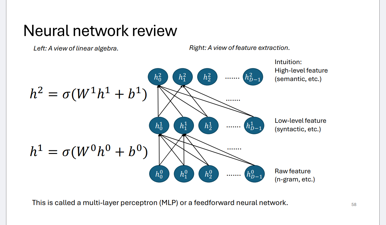

Bag of words

A simple way to encode a sentence: a |V|-dim vector, the i-th dimension indicates whether the i-th word in V(vocabulary) exists in x

h=Wx embed

注意：The difference with LSA and word2vec is that here the word embedding matrix is treated as part (the first layer) of the parameters of the NN model. But indeed, you can use word2vec/LSA (trained on larger data without label) to initialize this matrix.

\[\sigma'(z) = \sigma(z) \cdot (1 - \sigma(z))\]

A linear transform \(y=Wx\), stacking linear transfroms is still a linear transform.

Back-Propagation

Chain Rule

\[z = Wh + b \]

\[ \frac{\partial z}{\partial h}=W \]

\[ \frac{\partial z}{\partial W}=h^\top \]

\[ \frac{\partial z}{\partial b}=I \]

one hot：只有真实的label为1，其他的全0

\[\frac{\partial \mathcal{L}_{\text{CE}}(\mathbf{y}|\mathbf{x})}{\partial \mathbf{z}} = \frac{\partial (-\log(\text{softmax}(\mathbf{z}))[\mathbf{y}])}{\partial \mathbf{z}} = \text{softmax}(\mathbf{z}) - \mathbf{\tilde{y}}\]

proof： \(\mathcal{L}(\mathbf{z}, \mathbf{\tilde{y}}) = -\sum_{j=1}^K \tilde{y}_j \log(\hat{y}_j)\)

\(\mathbf{\hat{y}} = \text{softmax}(\mathbf{z})\)。其中 \(\hat{y}_j = \frac{e^{z_j}}{\sum_{k=1}^K e^{z_k}}\)。 * 真实标签： \(\mathbf{\tilde{y}}\)，假设真实标签是 \(c\)，则 \(\tilde{y}_c = 1\)，其余 \(\tilde{y}_j = 0\)。 * 交叉熵损失： \(\mathcal{L}(\mathbf{z}, \mathbf{\tilde{y}}) = -\sum_{j=1}^K \tilde{y}_j \log(\hat{y}_j)\)。 * 因为 \(\mathbf{\tilde{y}}\) 是 one-hot 向量，所以上式简化为：\(\mathcal{L} = -\log(\hat{y}_c) = -\log\left(\frac{e^{z_c}}{\sum_{k=1}^K e^{z_k}}\right)\)。

\(i\) 是正确分类 \(c\) 的索引（即 \(i=c\)）

\[\frac{\partial \mathcal{L}}{\partial z_c} = \frac{\partial}{\partial z_c} \left[ -\log\left(\frac{e^{z_c}}{\sum_{k=1}^K e^{z_k}}\right) \right]\]

利用对数性质 \(\log(A/B) = \log A - \log B\)： \[\mathcal{L} = -z_c + \log\left(\sum_{k=1}^K e^{z_k}\right)\]

求导： \[\frac{\partial \mathcal{L}}{\partial z_c} = \frac{\partial}{\partial z_c}(-z_c) + \frac{\partial}{\partial z_c}\left(\log\left(\sum_{k=1}^K e^{z_k}\right)\right)\] \[\frac{\partial \mathcal{L}}{\partial z_c} = -1 + \underbrace{\frac{1}{\sum_{k=1}^K e^{z_k}}}_{\text{外层导数}} \cdot \underbrace{e^{z_c}}_{\text{内层导数}}\]

回代 Softmax 的定义 \(\hat{y}_c = \frac{e^{z_c}}{\sum_{k=1}^K e^{z_k}}\)： \[\frac{\partial \mathcal{L}}{\partial z_c} = -1 + \hat{y}_c\]

因为 \(i=c\)，所以 \(\tilde{y}_i = 1\)。 \[\frac{\partial \mathcal{L}}{\partial z_i} = \hat{y}_i - 1 = \hat{y}_i - \tilde{y}_i\]

\(i\) 不是正确分类的索引（即 \(i \neq c\)）

\[\frac{\partial \mathcal{L}}{\partial z_i} = \frac{\partial}{\partial z_i} \left[ -z_c + \log\left(\sum_{k=1}^K e^{z_k}\right) \right]\]

求导（注意 \(-z_c\) 项对 \(z_i\) 的导数为 0）： \[\frac{\partial \mathcal{L}}{\partial z_i} = 0 + \underbrace{\frac{1}{\sum_{k=1}^K e^{z_k}}}_{\text{外层导数}} \cdot \underbrace{e^{z_i}}_{\text{内层导数}}\]

回代 Softmax 的定义 \(\hat{y}_i = \frac{e^{z_i}}{\sum_{k=1}^K e^{z_k}}\)： \[\frac{\partial \mathcal{L}}{\partial z_i} = \hat{y}_i\]

因为 \(i \neq c\)，所以 \(\tilde{y}_i = 0\)。 \[\frac{\partial \mathcal{L}}{\partial z_i} = \hat{y}_i - 0 = \hat{y}_i - \tilde{y}_i\]

Dropout

训练的时候随机失活： 在处理每个 mini-batch 数据时，神经网络中的每个神经元单元（Unit）（及其所有传入和传出的连接）都会以一个预设的概率 \(p\) 被随机地“丢弃”或失活。
At test time, all units are present, but with weights scaled by p (i.e. w becomes pw)

parallel computing: For a minibatch of input, we can concat them into a input matrix. Matrix-vector operation now becomes matrix-matrix operation.

NNLM

feed forward neural network

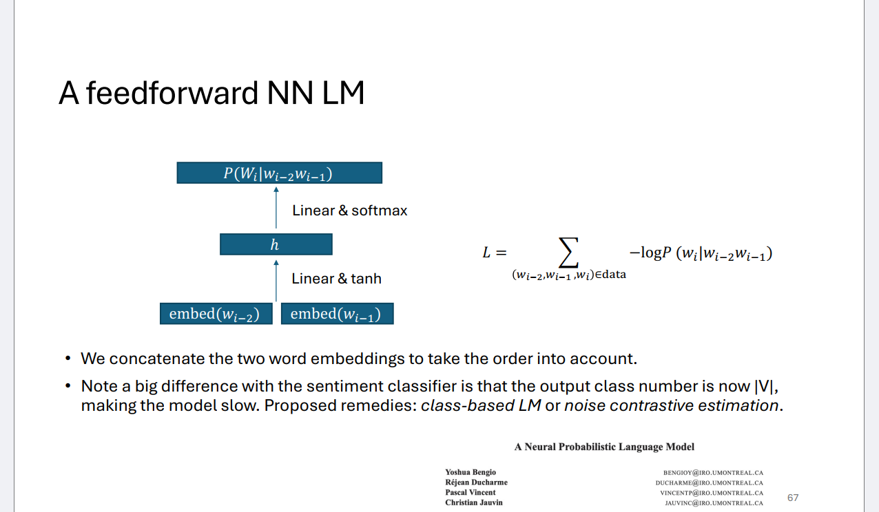
Note a big difference with the sentiment classifier is that the output class number is now |V|, making the model slow.

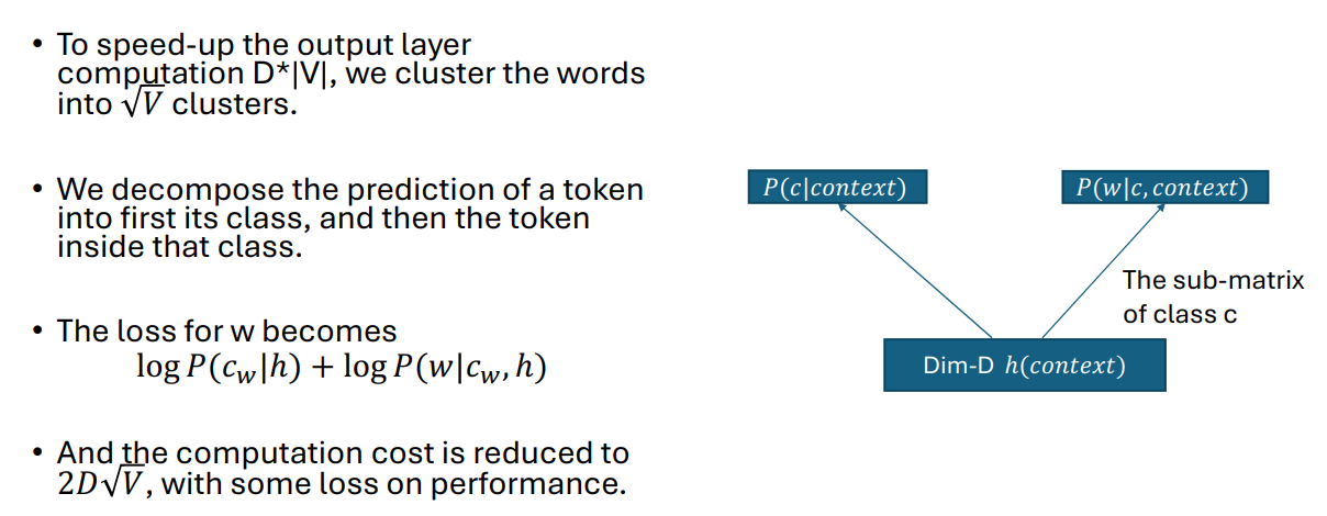
class-based neural network

RNN

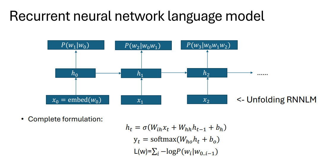
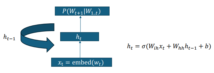
better long distance dependence： hidden states， shared \(W_ih\) and \(W_hh\)

Back propagation through time

problem: gradient explode/ vanish

标准的 RNN 隐藏状态计算是：\(h_t = \text{activation}(W_{hh} h_{t-1} + W_{ih} x_t)\)。

这里简化为：\(h_t \approx W_{hh} h_{t-1} + W_{ih} x_t\)。

从 \(h_t\) 到 \(h_{t-1}\) 的梯度 \(\frac{\partial h_t}{\partial h_{t-1}} \approx W_{hh}\)。

\[\frac{\partial L_t}{\partial h_1} \approx W_{hh}^{T^{t-1}} \frac{\partial L_t}{\partial h_t}\]

t-1次连乘导致梯度爆炸/消失

Gradient exploding is more serious because it makes training impossible，因为梯度无限大了

解决方案：gradient clipping，set the maximum norm of gradient to be \(\gamma\).

parallel of rnn：parallel across scentence

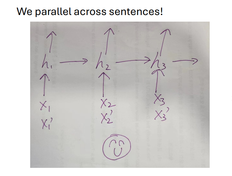
parallel traning: use padding to get same scentence length

you can also design a cnn to deal with variable seqlen

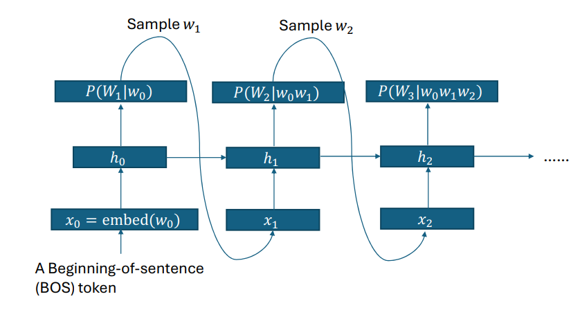
autoregressive LM

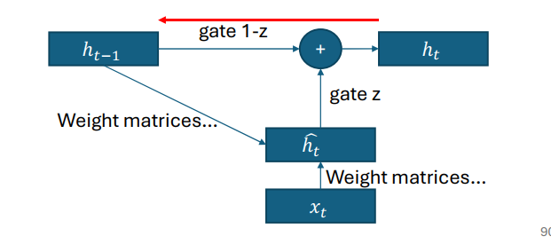
Gated recurrent unit

\[h_t = z_t \odot \hat{h}_t + (1 - z_t) \odot h_{t-1}\]

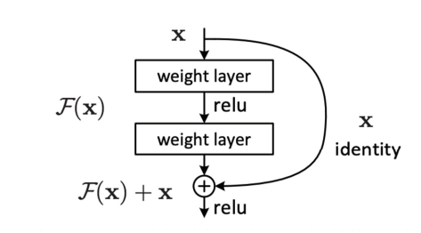
resnet

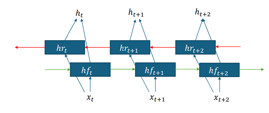
Bidirectional RNN

cannot be applied to AR-LM, because we cannot uitilize the information from the future. 最终的hidden state必须等到所有计算全部结束之后才能完成。

Encoder-decoder

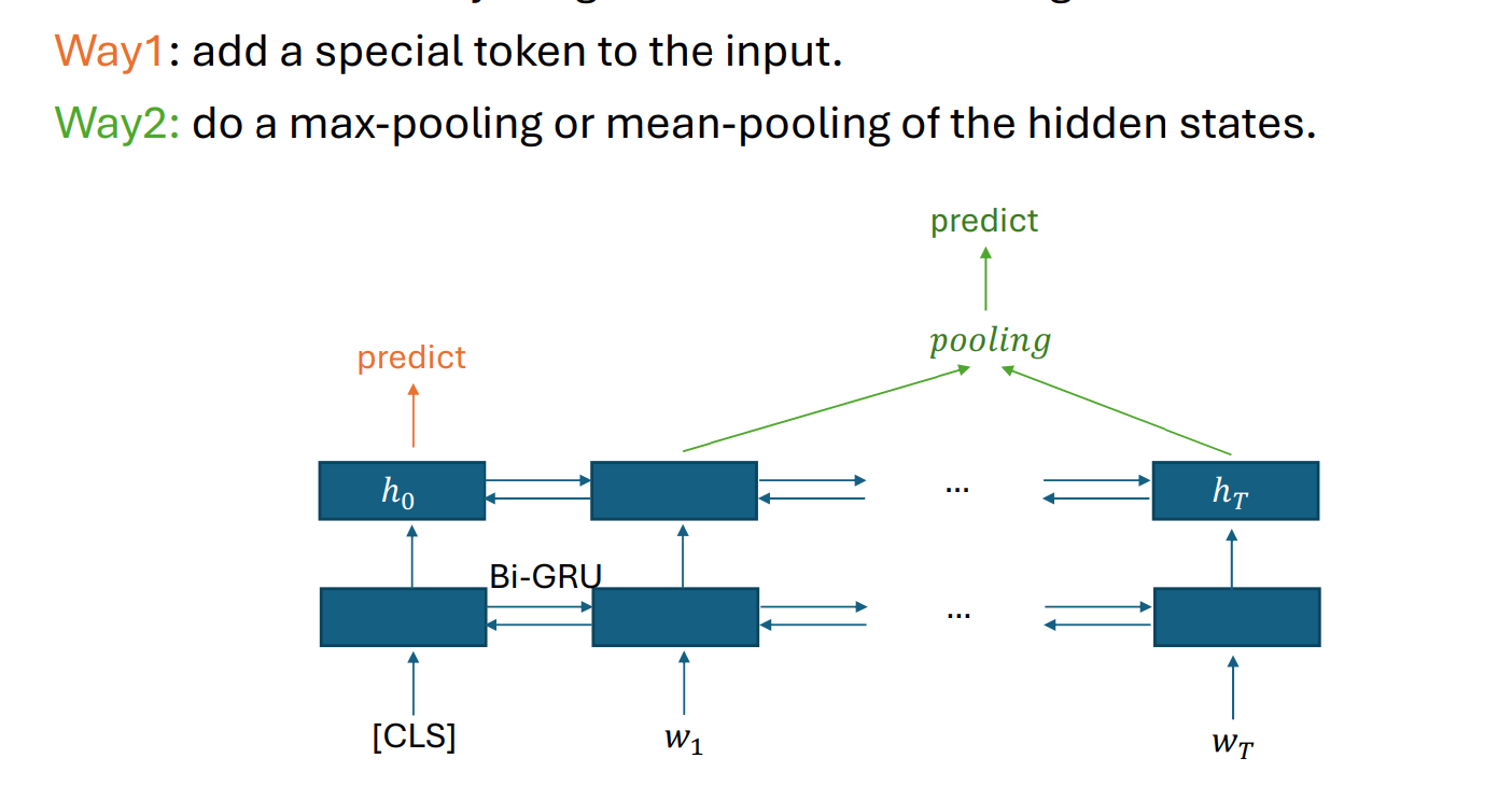
scentence-encoding: 句子最开始加一个特殊的token，这个主要利用的是反向的h0

We can use a bi-rnn encoder for the input sequence, and use a uni-rnn decoder for the output.

attention

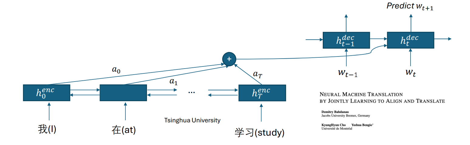
步骤一：计算对齐分数 (Alignment Score) \[\tilde{a}_i = (h_i^{enc})^T W_a h_{t-1}^{dec}\] 步骤二：计算注意力分布 (Attention Distribution) \[a = \text{softmax}(\tilde{a})\] 步骤三：计算上下文向量 (Context Vector) \[c_t = \sum_{i} a_i h_i^{enc}\]

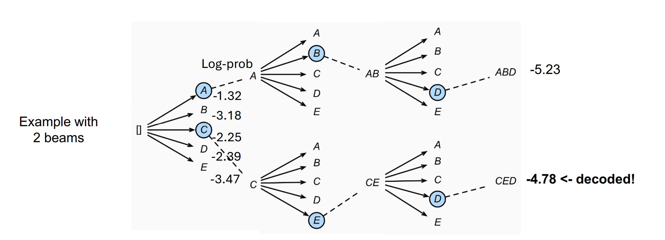
greedy decoding

autoregressive，每一次都选择局部最优的，所以不一定是全局最优的

beam search decoding

// 步骤 1: 初始化
// 初始化集束 (beams)。集束是一个列表，存储当前得分最高的 B 个候选序列。
// 格式：[(序列, 累积对数概率得分)]
beams = [["<s>", 0]] 
// 初始序列为起始符号 "<s>"，累积得分为 0。

// 步骤 2: 迭代生成序列
// L 是目标序列的最大长度。循环从 t=1（生成第一个词）到 L。
for t from 1 to L:
    // 初始化一个新的集束列表，用于存储当前时间步 t 扩展后的所有新序列。
    new_b = [] 
    
    // 遍历当前集束中的所有 B 个候选序列。
    for b in beams:
        // 解构当前候选序列：his 是历史序列，score 是它的累积对数概率得分。
        his, score = b[0], b[1]
        
        // 使用语言模型 (LM) 预测下一个词的概率分布。
        // logprob 存储基于 his 得到的词汇表所有词的对数概率。
        logprob = LM-NextPredict[his] 
        
        // 从 logprob 中选择概率最高的 k=B 个词汇及其对数概率。
        // idx_s: 这 B 个词汇在词汇表中的索引。
        // logprob_s: 这 B 个词汇对应的对数概率。
        idx_s, logprob_s = top-k(logprob, k=B)
        
        // 步骤 3: 扩展序列并计算新得分
        // 遍历这 B 个最佳的下一个词汇。
        for j from 0 to (B-1):
            // 扩展序列：将新的最佳词 V[idx_s[j]] 添加到历史序列 his 后面。
            // V 是词汇表 (Vocabulary)。
            // 更新得分：新得分 = 旧得分 + 新词汇的对数概率 (因为 log(P1*P2) = log(P1)+log(P2))。
            new_b.append((his + V[idx_s[j]], score + logprob_s[j]))
    
    // 步骤 4: 筛选和更新集束
    // 对 new_b 中的所有序列（当前有 B*B 个）按得分（score）进行降序排序。
    // 只保留得分最大的 B 个序列。
    sort and only keep B sequences in new_b with largest score.
    
    // 用筛选后的 B 个最佳序列更新 beams，进入下一轮迭代。
    beams = new_b

// 步骤 5: 返回结果
// 循环结束后，beams 中存储了长度为 L 的 B 个最佳序列。
// 返回得分最高（排在第一位）的序列。
return beams[0]

关键；每一次一个node都会生成b个分支，但我们只保留得分最大的b个

belu metric for machine translation

\[ \text{precision}_n = \frac{\text{number of } n\text{-gram matches in reference}}{\text{number of } n\text{-grams in predicted}} \]

简洁惩罚用于惩罚那些比参考译文短的机器译文，以确保翻译的长度合理。

\[ \text{brevity-penalty} = \min \left\{ 1, \exp \left( 1 - \frac{|\text{reference}|}{|\text{predicted}|} \right) \right\} \]

BLEU 最终得分是简洁惩罚和几何平均 \(n\)-gram 精准度的乘积。

\[ \text{BLEU} = \text{brevity-penalty} \times \left( \prod_{n=1}^{4} \text{precision}_n \right)^{\frac{1}{4}} \]

creating paired data

Given a decent amount of bilingual data (X, Y) and a good amount monolingual data in target language Y.

• Q: What can you do to create more paired bilingual data?

• You can train a backward model Y->X, and conduct generation on the monolingual data. That’s called back translation.

GLUE benchmark

The General Language Understanding Evaluation , human level

SuperGLUE, harder

ELMo

ELMo (Embeddings from Language Models): build deep contextualized word representation.

Model: multilayer bidirectional LSTM

Objective: predict the next word in both directions independently; i.e., left-to-right and right-to-left

subword tokenization

• (1) Start with a unigram vocabulary of all characters in the data.

• (2) Each iteration: In the data, find the most frequent pair, merge it, and add to the vocabulary.

• (3) Stop when vocabulary is of pre-determined size (e.g., 50k).

Transformer

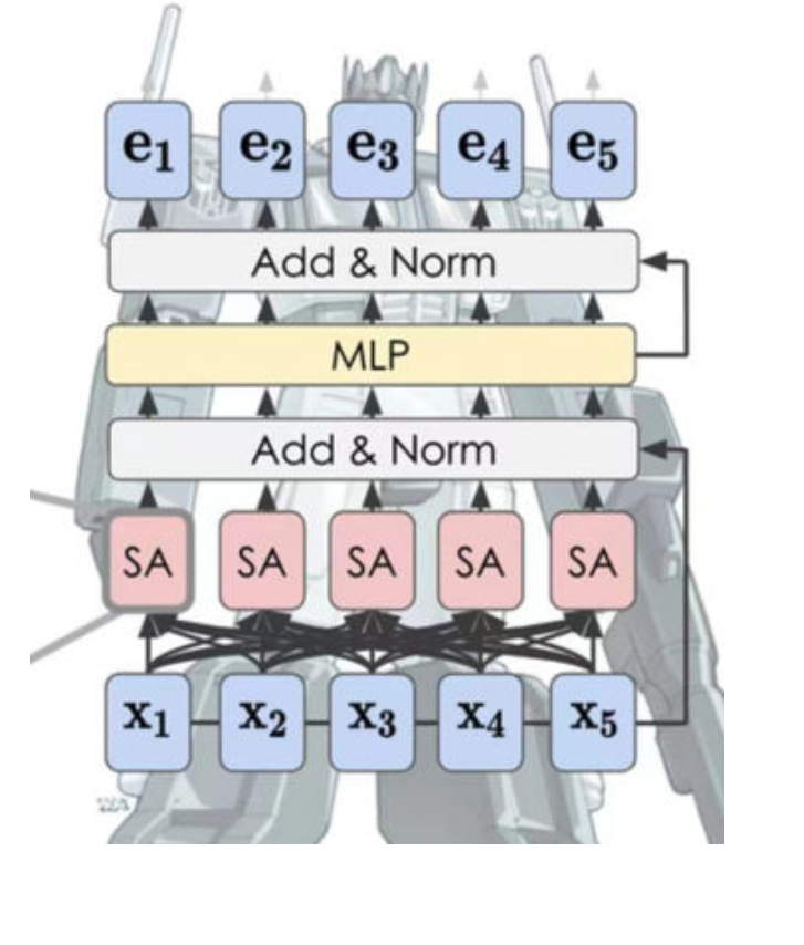
Self-attention

q, k, v 均为 Wx

计算第 \(i\) 个位置的查询向量 \(\mathbf{q}_i\) 对所有键向量 \(\mathbf{k}_*\)（其中 \(*\) 代表句子中的所有位置）的注意力权重的公式如下：

\[a_{i*} = \mathbf{softmax}\left(\frac{\mathbf{q}_i^\top \mathbf{k}_*}{\sqrt{\text{dim}_k}}\right)\]

divide \(\sqrt{\text{dim}_k}\), normalize the variance, achieve more stable and smooth softmax output.

\(Z = softmax(\frac{QK^\top}{\sqrt{dimk}})V\) parallel computation

layernorm

\[\mathbf{LayerNorm}(\mathbf{h}) = \alpha \cdot \frac{\mathbf{h} - \text{mean}(\mathbf{h})}{\text{std}(\mathbf{h})} + \beta\]

class LayerNorm(nn.Module):
    
    def __init__(self, features, eps=1e-6):
        super(LayerNorm, self).__init__()
        self.a_2 = nn.Parameter(torch.ones(features)) #参数
        self.b_2 = nn.Parameter(torch.zeros(features))
        self.eps = eps #一个很小的数，防止除以0

    def forward(self, x):
        # x:(seqlen,feature)
        mean = x.mean(-1, keepdim=True)
        std = x.std(-1, keepdim=True)
        return self.a_2 * (x - mean) / (std + self.eps) + self.b_2

conbined with resnet: \(h_{out}=F(layernorm(h))+h\)

batchnorm往往需要batchsize比较大，但当我们训大语言模型的时候batchsize可能达不到那么大。而且qkv的维度d是确定的，但seqlen不确定，所以layernorm更加适合sequence model。

multihead

每一个head一套qkv的权重矩阵，最后concat再linear

positional encoding

Without RNN, attention alone does not have order information!

Exercise: Given any \(\text{pos}\) vector and a fixed number \(k\), can you represent \(\text{pos} + k\) as a linear transform of \(\text{pos}\)?

Hint: \(\sin(A+B) = \sin A \cos B + \sin B \cos A\)

这里的 \(\text{pos}\) 是指位置 \(pos\) 的位置编码向量，而 \(\text{pos}+k\) 是指位置 \(pos+k\) 的位置编码向量。

假设位置编码向量的第 \(i\) 个维度分量定义如下： \[\text{PE}_{\text{pos}, i} = \sin(\omega_i \cdot \text{pos})\]

其中 \(\omega_i\) 是与维度 \(i\) 相关的固定频率项。

现在，我们来看位置 \(\text{pos}+k\) 的第 \(i\) 个分量： \[\text{PE}_{\text{pos}+k, i} = \sin(\omega_i \cdot (\text{pos} + k))\]

利用提示中的三角恒等式 \(\sin(A+B) = \sin A \cos B + \sin B \cos A\)，其中 \(A = \omega_i \cdot \text{pos}\)，\(B = \omega_i \cdot k\)：

\[\text{PE}_{\text{pos}+k, i} = \underbrace{\sin(\omega_i \cdot \text{pos})}_{\text{PE}_{\text{pos}, i}} \cdot \underbrace{\cos(\omega_i \cdot k)}_{\text{固定常量}} + \underbrace{\cos(\omega_i \cdot \text{pos})}_{\text{PE}_{\text{pos}, i}^{\text{perp}}} \cdot \underbrace{\sin(\omega_i \cdot k)}_{\text{固定常量}}\]

\[\mathbf{PE}_{\text{pos}+k} = \mathbf{A}_k \cdot \mathbf{PE}_{\text{pos}}\]

lr warm-up and linear decay

We usually start with a large learning rate (lr), and then decay over time.

For transformer models, it is very useful to set a small warmup stage, where we first gradually increase lr from zero to the starting value.

Without this trick, training is likely to get stuck.

BERT

pretrained with self supervised training, no labels!

Two major objective used in BERT pretraining:

• Masked language modeling (MLM)

• Next sentence prediction (NSP)

MLM Masked language modeling

Randomly mask (via a [mask] token) 15% of the tokens in each sequence.

Ask the transformer model to predict the masked token on the top layer via standard cross-entropy loss.

特性	掩码语言建模 (MLM) - BERT	连续词袋模型 (CBOW) - Word2Vec
模型架构	深层 Transformer 编码器 (Deep Transformer Encoder)。	浅层神经网络 (Shallow Neural Network)。
训练目标	预测输入序列中被 `[MASK]` 标记随机替换的词元。	预测窗口内缺失的目标词语，根据其周围的上下文词语。
上下文利用	利用双向上下文 (左侧和右侧) 以及整个序列的信息。依赖 Transformer 的自注意力机制来捕捉远距离依赖。	仅利用固定大小窗口内的上下文词语。将上下文词语视为“词袋”，通常通过求和或平均它们的向量来表示上下文。
词序敏感性	敏感。由于使用了 Transformer 架构和位置编码，模型知道词语的先后顺序。	不敏感。因为它将上下文词语视为一个“袋子”进行处理 (求和/平均)，丢失了词语的先后顺序信息。
输出结果	语境化/动态嵌入 (Contextualized/Dynamic Embeddings)。同一个词在不同句子中的含义不同，其向量也不同。	静态嵌入 (Static Embeddings)。无论出现在什么语境中，一个词语都只有一个固定的向量表示。
处理多义词	出色。能区分多义词的不同含义（例如，“银行”作为金融机构和“河岸”的含义）。	较弱。无法区分多义词的不同含义，会为所有语境下的多义词学习同一个向量。

Problem: If we only add loss for masked tokens, then the transformer would not build good representations for nonmasked tokens.

For 10% of the time, we replace [M] with a random token.

For another 10% of the time, we do not change the original token.

80% remaining time, the mask token is used.

NSP Next Sentence Prediction

In addition to MLM, we also add a [CLS] token and ask BERT to predict whether sentence2 is the next sentence of sentence1.

[CLS] 来分类，[SEP] 来分割句子

finetune

BERT finetuning cont.

• After pretraining, we slightly modify the top layers of BERT and tune it on downstream tasks

top layer: 输出 \(T\) 的层

efficient approach

ELECTRA

生成器 (Generator)

工作原理： 它通常是一个小型的掩码语言模型 (MLM)。
输入处理： 它首先像 BERT 那样，对输入句子进行掩码（如将 "the chef cooked the meal" 变为 "the chef [MASK] the meal"）。
输出： 它预测被掩码的词元，并用这些貌似合理 (plausible) 的预测替代原句子中的一些词元。
- 示例： 原始句子中的 cooked 被 [MASK]，生成器可能会预测出 ate，然后用 ate 替换原词。

判别器 (Discriminator) - ELECTRA 模型本身

输入： 接收被生成器替换（损坏） 过的输入序列。
这是一个二元分类任务：对每个词元 \(x_i\)，预测 \(P(\text{IsReplaced}|x_i)\)。

This new pre-training task is more efficient than MLM because the task is defined over all input tokens rather than just the small subset that was masked out.

Longformer Sliding Window Attention

每个 Token 的计算量： 对于序列中的任意一个 token（查询 Q），它只需要计算与它局部窗口 \(w\) 内的其他 \(w\) 个 token（键 K）的注意力得分, \(O(w)\)。总计算量 \(\approx n \times O(w) = O(n \cdot w)\)。

For an embedding on layer L, what’s its receptive field? (how many input tokens does it cover?)

Lxw

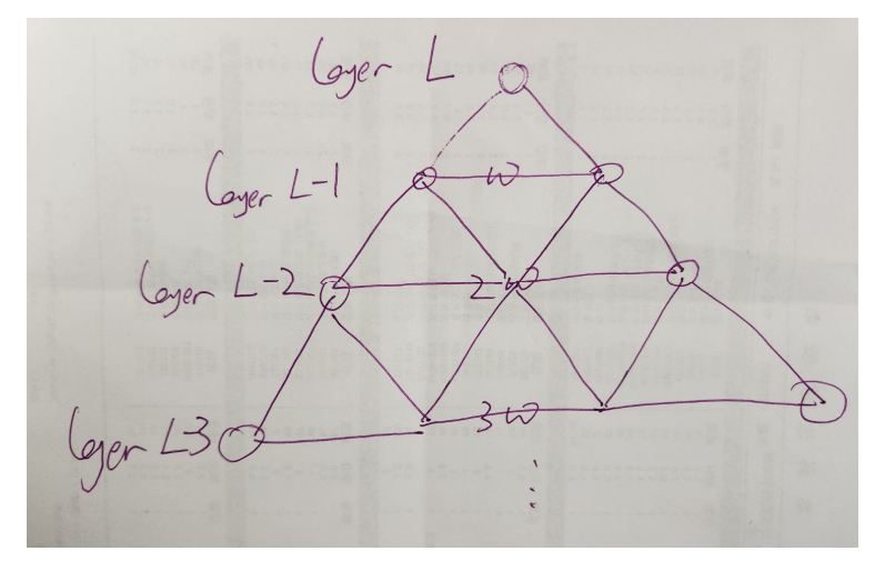
Combined with dilated sliding window

We can add gaps in the window to make it even wider with the same amount of compute(捕捉长距离依赖)

We can use a combination of 2 heads of dilated and other heads with local sliding window.（用multihead实现短距离长距离结合）

VAE-LM（不考）

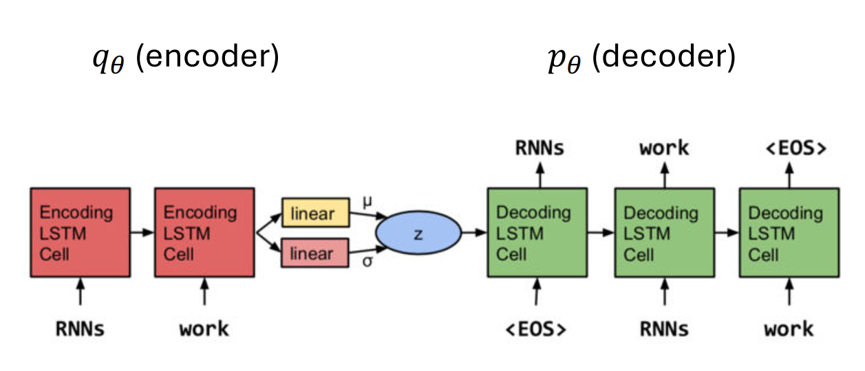
组件	名称	功能	结构
\(q_{\phi}\) (Encoder)	编码器/后验模型	接收输入句子 \(\mathbf{x}\)，将它压缩成一个潜在语义向量 \(\mathbf{z}\) 的分布。	1. \(\text{RNNs}\) (LSTM Cell): 编码整个句子 \(\mathbf{x}\)。 2. Linear Layers: 根据 \(\text{RNN}\) 的最终隐藏状态，输出潜变量 \(\mathbf{z}\) 分布的参数 \(\mu\) (均值) 和 \(\sigma\) (方差)。
\(\mathbf{z}\)	潜在变量 (Latent Variable)	一个连续的低维向量，代表整个句子的全局语义。	从 \(\mathbf{z}\) 的分布中采样得到。
\(p_{\theta}\) (Decoder)	解码器/生成模型	接收 \(\mathbf{z}\) 作为输入，并逐字生成（重构）句子 \(\mathbf{x}\)。	1. \(\text{RNNs}\) (LSTM Cell): 接收 \(\mathbf{z}\) 作为初始状态或输入。 2. 生成过程: 从起始符号（如 `<EOS>` 在图中似乎被误置，通常是 `<BOS>` 或 \(\mathbf{z}\)）开始，逐步生成 \(\text{work} \rightarrow \text{work} \rightarrow \text{<EOS>}\)。

后验 (\(q_{\phi}\)) 和先验 (\(p(\mathbf{z})\)) 分布： 图中明确指出，先验分布 \(p(\mathbf{z})\) 和后验分布 \(q_{\phi}(\mathbf{z} | \mathbf{x})\) 都是高斯分布 (Gaussian)，且通常是对角协方差矩阵（diagonal），这意味着它们在潜空间中是可参数化的。

🚀 生成 (Generation) 过程

生成新句子时，我们只使用解码器 \(p_{\theta}\)：

Sample \(\mathbf{z}\) from prior \(p(\mathbf{z})\): 从一个简单的先验分布（如标准正态分布 \(\mathcal{N}(\mathbf{0}, \mathbf{I})\)）中随机采样一个潜在语义向量 \(\mathbf{z}\)。这个 \(\mathbf{z}\) 就是我们希望生成句子所拥有的意图或主题。
Sample \(\mathbf{x}\) from our generative model \(p_{\theta}(\mathbf{x} | \mathbf{z})\): 将这个采样的 \(\mathbf{z}\) 喂给解码器，解码器 \(\text{RNN}\) 就会逐词生成句子 \(\mathbf{x}\)，直到生成结束符号 (\(\text{<EOS>}\))。

📈 训练目标：\(\text{VAE}\) "\(\text{ELBO}\)" (最大化)

\[ \mathcal{L}(\theta; \mathbf{x}) = \underbrace{-\text{KL}(q_{\phi}(\mathbf{z} | \mathbf{x}) \| p(\mathbf{z}))}_{\text{I. KL Divergence (Regularization Term)}} + \underbrace{\mathbb{E}_{q_{\phi}(\mathbf{z} | \mathbf{x})}[\log p_{\theta}(\mathbf{x} | \mathbf{z})]}_{\text{II. Expectation of Log-Likelihood (Reconstruction Term)}} \]

I. \(\text{KL}\) 散度项（\(-\text{KL}(\dots)\)）
\[-\text{KL}(q_{\phi}(\mathbf{z} | \mathbf{x}) \| p(\mathbf{z}))\]
- 作用： 这是一个正则化项，它衡量了编码器输出的后验分布 \(q_{\phi}(\mathbf{z} | \mathbf{x})\) 与简单的先验分布 \(p(\mathbf{z})\) 之间的差异。
II. 重构项 (\(\mathbb{E}[\log p_{\theta}(\mathbf{x} | \mathbf{z})]\))
\[\mathbb{E}_{q_{\phi}(\mathbf{z} | \mathbf{x})}[\log p_{\theta}(\mathbf{x} | \mathbf{z})]\]
- 作用： 这是一个重构项，它衡量了解码器从潜在向量 \(\mathbf{z}\) 重构出原始句子 \(\mathbf{x}\) 的对数概率。
证据下界
\(\text{ELBO}\) 的值小于或等于数据的对数边缘似然 \(\log p(\mathbf{x})\)： \[\mathcal{L}(\theta; \mathbf{x}) \leq \log p(\mathbf{x})\] 因此，最大化 \(\mathcal{L}(\theta; \mathbf{x})\) 就是在最大化 \(\log p(\mathbf{x})\) 的一个下界，从而间接优化了整个模型。

📈 \(\text{ELBO}\) 推导过程解释

推导的目标是找到 \(\log p(\mathbf{x})\) 的一个下界，我们称之为 \(\mathcal{L}(\theta; \mathbf{x})\) 或 \(\text{ELBO}\)。

\[ \ln p(\mathbf{x}) = \ln \int_{\mathbf{z}} p(\mathbf{x}, \mathbf{z}) d\mathbf{z} \]

\[ = \ln \int_{\mathbf{z}} p(\mathbf{x}, \mathbf{z}) \frac{q(\mathbf{z} | \mathbf{x})}{q(\mathbf{z} | \mathbf{x})} d\mathbf{z} \]

\[ \ge \mathbb{E}_{q(\mathbf{z} | \mathbf{x})}\left[\ln \frac{p(\mathbf{x}, \mathbf{z})}{q(\mathbf{z} | \mathbf{x})}\right] \]

说明： 这是推导的关键一步。由于 \(\ln(\cdot)\) 是一个凹函数 (concave function)，根据 詹森不等式 (Jensen's Inequality)，对于任何随机变量 \(Y\)： \[\ln(\mathbb{E}[Y]) \ge \mathbb{E}[\ln(Y)]\]

\[ = \mathbb{E}_{q(\mathbf{z} | \mathbf{x})}\left[\ln \frac{p(\mathbf{x}, \mathbf{z})}{q(\mathbf{z} | \mathbf{x})}\right] \] \[ = \mathbb{E}_{q(\mathbf{z} | \mathbf{x})}\left[\ln \frac{p(\mathbf{x} | \mathbf{z}) p(\mathbf{z})}{q(\mathbf{z} | \mathbf{x})}\right] \]

\[ = \mathbb{E}_{q(\mathbf{z} | \mathbf{x})}\left[\ln p(\mathbf{x} | \mathbf{z})\right] + \mathbb{E}_{q(\mathbf{z} | \mathbf{x})}\left[\ln \frac{p(\mathbf{z})}{q(\mathbf{z} | \mathbf{x})}\right] \]

\[ = \mathbb{E}_{q(\mathbf{z} | \mathbf{x})}\left[\ln p(\mathbf{x} | \mathbf{z})\right] - \int_{\mathbf{z}} q(\mathbf{z} | \mathbf{x}) \ln \frac{q(\mathbf{z} | \mathbf{x})}{p(\mathbf{z})} d\mathbf{z} \] \[ = \text{likelihood} - \mathbb{D}_{\text{KL}}[q(\mathbf{z} | \mathbf{x}) \| p(\mathbf{z})] \]

在 \(\text{VAE}\) 训练中，我们通过最大化这个 \(\text{ELBO}\) 目标函数，间接实现了对真实数据分布 \(p(\mathbf{x})\) 的建模。

从 KL 散度的定义开始： \[D_{KL}(q_{\phi}(\mathbf{z}|\mathbf{x}) || p_{\theta}(\mathbf{z}|\mathbf{x})) = E_{q_{\phi}(\mathbf{z}|\mathbf{x})} \left[ \log \frac{q_{\phi}(\mathbf{z}|\mathbf{x})}{p_{\theta}(\mathbf{z}|\mathbf{x})} \right]\]

将对数中的除法分解为减法： \[D_{KL} = E_{q_{\phi}(\mathbf{z}|\mathbf{x})} \left[ \log q_{\phi}(\mathbf{z}|\mathbf{x}) \right] - E_{q_{\phi}(\mathbf{z}|\mathbf{x})} \left[ \log p_{\theta}(\mathbf{z}|\mathbf{x}) \right]\]

根据贝叶斯定理 \(p(\mathbf{z}|\mathbf{x}) = \frac{p(\mathbf{x}, \mathbf{z})}{p(\mathbf{x})}\)，我们有 \(\log p(\mathbf{z}|\mathbf{x}) = \log p(\mathbf{x}, \mathbf{z}) - \log p(\mathbf{x})\)。代入上式：

\[D_{KL} = E_{q_{\phi}(\mathbf{z}|\mathbf{x})} \left[ \log q_{\phi}(\mathbf{z}|\mathbf{x}) \right] - E_{q_{\phi}(\mathbf{z}|\mathbf{x})} \left[ \log p_{\theta}(\mathbf{x}, \mathbf{z}) - \log p_{\theta}(\mathbf{x}) \right]\]

将期望中的 \(\log p_{\theta}(\mathbf{x})\) 移出（因为它与 \(\mathbf{z}\) 无关，期望值就是它本身）：

重新排列各项： \[\log p_{\theta}(\mathbf{x}) = E_{q_{\phi}(\mathbf{z}|\mathbf{x})} \left[ \log p_{\theta}(\mathbf{x}, \mathbf{z}) \right] - E_{q_{\phi}(\mathbf{z}|\mathbf{x})} \left[ \log q_{\phi}(\mathbf{z}|\mathbf{x}) \right] + D_{KL}(q_{\phi}(\mathbf{z}|\mathbf{x}) || p_{\theta}(\mathbf{z}|\mathbf{x}))\]

最后，我们将前两项合并，得到 ELBO 的定义： \[\mathcal{L}(\theta, \phi) = E_{q_{\phi}(\mathbf{z}|\mathbf{x})} \left[ \log \frac{p_{\theta}(\mathbf{x}, \mathbf{z})}{q_{\phi}(\mathbf{z}|\mathbf{x})} \right]\]

所以，我们最终得到这个关键等式： \[\log p(\mathbf{x}) = \mathcal{L}(\theta, \phi) + D_{KL}(q_{\phi}(\mathbf{z}|\mathbf{x}) || p_{\theta}(\mathbf{z}|\mathbf{x}))\]

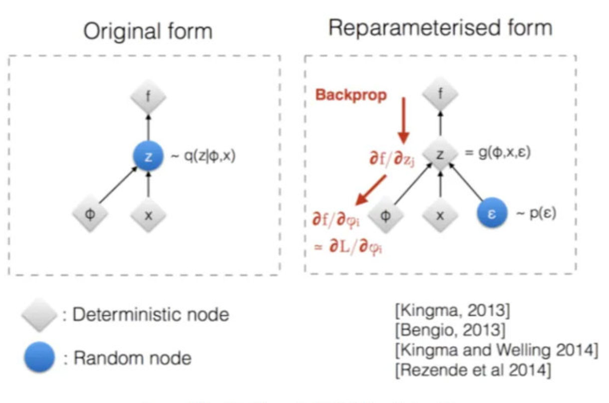
重参数

the second term involves a sampling operation from the parameterized q, which we can not directly back-prop

在引入重新参数化技巧之前，我们计算重构项的梯度是这样的：

\[\nabla_{\phi} E_{q_{\phi}(\mathbf{z}|\mathbf{x})} [\log p_{\theta}(\mathbf{x}|\mathbf{z})]\]

当我们使用蒙特卡洛采样来近似这个期望时：

\[\nabla_{\phi} \left( \frac{1}{M} \sum_{m=1}^{M} \log p_{\theta}(\mathbf{x}|\mathbf{z}^{(m)}) \right) \quad \text{其中 } \mathbf{z}^{(m)} \sim q_{\phi}(\mathbf{z}|\mathbf{x})\]

问题核心在于：

采样过程 (\(\mathbf{z} \sim q_{\phi}(\mathbf{z}|\mathbf{x})\)) 是一个离散的、不可逆的随机操作。
它就像一个黑箱，输入是参数 \(\phi\)（决定了 \(q\) 的 \(\mu\) 和 \(\sigma\)），输出是样本 \(\mathbf{z}\)。从数学上讲，这个从 \(\phi\) 到 \(\mathbf{z}\) 的映射是不可导的。
因此，我们无法利用链式法则计算 \(\mathbf{z}\) 对 \(\phi\) 的梯度 \(\frac{\partial \mathbf{z}}{\partial \phi}\)，也就无法将损失函数的梯度 \(\frac{\partial \mathcal{L}}{\partial \mathbf{z}}\) 传递回 \(\phi\)。

重新参数化技巧就是通过重写随机变量的生成过程，将随机性（\(\epsilon\)）和参数依赖性 (\(\phi\) 通过 \(\mu, \sigma\)) 分离，从而创建一条可导的路径 (pathwise gradient)：

\[\mathbf{z} = \mu(\mathbf{x}, \phi) + \sigma(\mathbf{x}, \phi) \odot \epsilon\]

现在的计算图是：

\(\phi \to (\mu, \sigma)\) (确定性，可导)
\((\mu, \sigma)\) 和 \(\epsilon\) (随机但独立于 \(\phi\)) \(\to \mathbf{z}\) (确定性函数 \(g\)，可导)
\(\mathbf{z} \to \log p(\mathbf{x}|\mathbf{z})\) (确定性，可导)
\(\log p(\mathbf{x}|\mathbf{z}) \to \mathcal{L}\)

由于 \(\mathbf{z}\) 现在是 \(\phi\) 的一个确定性函数（通过 \(\mu\) 和 \(\sigma\)），我们可以直接使用链式法则求导：

\[\frac{\partial \mathcal{L}}{\partial \phi} = \frac{\partial \mathcal{L}}{\partial \mathbf{z}} \frac{\partial \mathbf{z}}{\partial \mu} \frac{\partial \mu}{\partial \phi} + \frac{\partial \mathcal{L}}{\partial \mathbf{z}} \frac{\partial \mathbf{z}}{\partial \sigma} \frac{\partial \sigma}{\partial \phi}\]

注：\(\frac{\partial \mathbf{z}}{\partial \sigma} =\epsilon\)

optimization challenge

KL term quickly decrease to zero (throwing away latent information)

Comparing to the second term, the KL-prior term is easier to optimize (why?).

• The RNN decoder is strong and has ground-truth history in its input.

1. KL 代价退火 (KL Cost Annealing) 🌡️

方法： 在目标函数中，为 KL 散度项添加一个可变权重 \(\beta\)。
- 在训练开始时，设置 \(\beta\) 接近或等于零。
- 随着训练的进行，\(\beta\) 逐渐增加，直到达到 1。
数学形式： \[\mathcal{L}(\theta; \vec{x}) = \mathbb{E}[\log p_\theta(\vec{x}|\vec{z})] - \beta \cdot \text{KL}(q_\phi(\vec{z}|\vec{x})||p(\vec{z}))\]
直觉解释：
1. 早期 ( \(\beta \approx 0\) ): 目标函数几乎只剩下重构项。这给了编码器和解码器充足的机会，去学习一个最大化信息量的潜在表示 \(\vec{z}\)，而不必担心 \(\vec{z}\) 是否接近先验分布 \(p(\vec{z})\)。
2. 后期 ( \(\beta \to 1\) ): KL 项的权重逐渐增大，开始发挥其正则化作用，迫使学习到的潜在分布 \(q_\phi(\vec{z}|\vec{x})\) 接近先验 \(p(\vec{z})\)。
效果： 这种方法有效地让模型先“学会说话”（学习有用的 \(\vec{z}\)），然后再“规范语法”（满足 KL 约束），从而避免了 \(\vec{z}\) 在训练初期就被优化器轻易抛弃。

2. 输入词丢弃 (Input Word Dropping) ✂️

方法： 这是一种直接削弱解码器的方法。
- 在训练时，随机地移除部分或全部用于教师强制的 Ground-Truth 历史词（即 \(x_{t-1}\)）。forcing the model to rely on the latent vector。 ---

3. 词袋损失 (Bag-of-Words Loss, BoW Loss) 🛍️

方法： 除了标准的序列重构损失外，并行地训练一个辅助解码器（或者在主解码器中增加一个分支）来预测输入 \(\vec{x}\) 的词袋表示 (Bag-of-Words, BoW)。
- 词袋表示： 是一个向量，只包含 \(\vec{x}\) 中每个词出现的次数，而忽略词的顺序（即非序列信息）。
- 这个 BoW 损失旨在确保 \(\vec{z}\) 至少编码了 \(\vec{x}\) 的内容信息，即使没有编码顺序信息。

#NLP

黎明之前：Transformer之前的自然语言处理

http://example.com/2025/12/12/nlp2/

作者

瑾瑜當年

发布于

2025年12月12日

许可协议

破晓之刻：Transformer的诞生与自然语言处理前沿上一篇

老派自然语言处理之必要下一篇

黎明之前：Transformer之前的自然语言处理

Review

KLD

⚖️ \(D_{KL}(P_D \| P_M)\) 的直觉：模式覆盖 (Mode-Covering)

核心直觉：害怕错过（对 \(P_D\) 的高密度区敏感）

⚔️ \(D_{KL}(P_M \| P_D)\) 的直觉：模式搜索 (Mode-Seeking)

核心直觉：害怕犯错（对 \(P_D\) 的低密度区敏感）

Multi-class classification

NN Basics

Bag of words

h=Wx embed

Back-Propagation

\(i\) 是正确分类 \(c\) 的索引（即 \(i=c\)）

\(i\) 不是正确分类的索引（即 \(i \neq c\)）

Dropout

NNLM

feed forward neural network

class-based neural network

RNN

autoregressive LM

Gated recurrent unit

Bidirectional RNN

Encoder-decoder

attention

greedy decoding

beam search decoding

belu metric for machine translation

creating paired data

GLUE benchmark

ELMo

subword tokenization

Transformer

Self-attention

layernorm

multihead

positional encoding

lr warm-up and linear decay

BERT

MLM Masked language modeling

NSP Next Sentence Prediction

finetune

efficient approach

ELECTRA

Longformer Sliding Window Attention

VAE-LM（不考）

🚀 生成 (Generation) 过程

📈 训练目标：\(\text{VAE}\) "\(\text{ELBO}\)" (最大化)

I. \(\text{KL}\) 散度项（\(-\text{KL}(\dots)\)）

II. 重构项 (\(\mathbb{E}[\log p_{\theta}(\mathbf{x} | \mathbf{z})]\))

证据下界

📈 \(\text{ELBO}\) 推导过程解释

重参数

optimization challenge

1. KL 代价退火 (KL Cost Annealing) 🌡️

2. 输入词丢弃 (Input Word Dropping) ✂️

3. 词袋损失 (Bag-of-Words Loss, BoW Loss) 🛍️